> ## Documentation Index
> Fetch the complete documentation index at: https://docs.ntop.com/llms.txt
> Use this file to discover all available pages before exploring further.
# How to use Conic and Cubic Bézier blocks
## **Applies to:**
* #### [**Conic**](#h-01k776vxq0r3jcvwtjp5b1cq2z)
* #### [**Cubic Bézier**](#h-01k776vxqdcf90hc45xd5vkg2p)
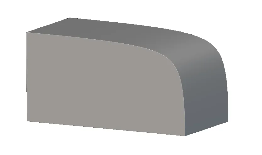
**Conic** and **Cubic Bézier** blocks are used for:
* Designing aerodynamic profiles for wings, fuselages, and other vehicle bodies.
* Modeling smooth transitions in components like ducts, inlets, and nozzles to manage fluid flow.
* Creating architectural features like arches and curved facades.
## **Procedure:**
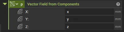
1. Create a 3D Position **Vector Field from Components** block (x,y, and z). This represents the spatial coordinates with units of length.
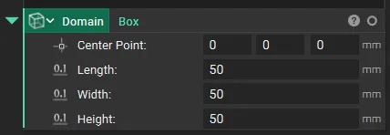
2. Create Design Space, which will be used to bound the Conic sections. In this example, we will use **Box**.
### **Conic**
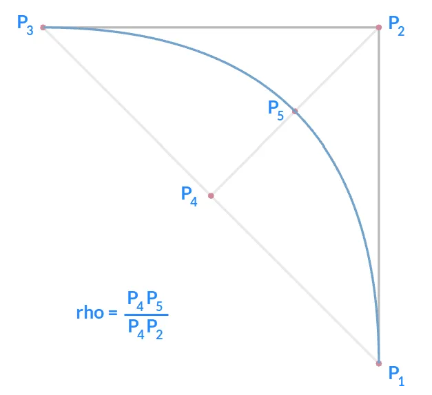
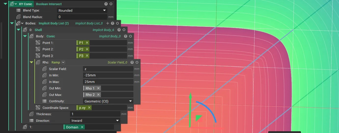
The Conic block creates a conic section (ellipse, parabola, or hyperbola) based on five inputs: Point 1 (P1), Point 2 (P2), Point 3 (P3), Rho (ρ), and the Coordinate Space.
Point 4 is the midpoint of the chord between Point 1 and Point 3. Point 5 is where the curve intersects the chord between Point 4 and Point 2.
* The **2D Vector Field** block creates a 2D vector field from scalar field components, defining the (x,y) coordinates of the control points. (Conceptually, you can imagine the z-component extending to infinity, (−∞,∞). If you need to visualize the 2D plane in a 3D space, use Lines.)
* We need three points to control our **Conic** section, so we will create three different 2D Vector Fields for P1, P2, and P3.
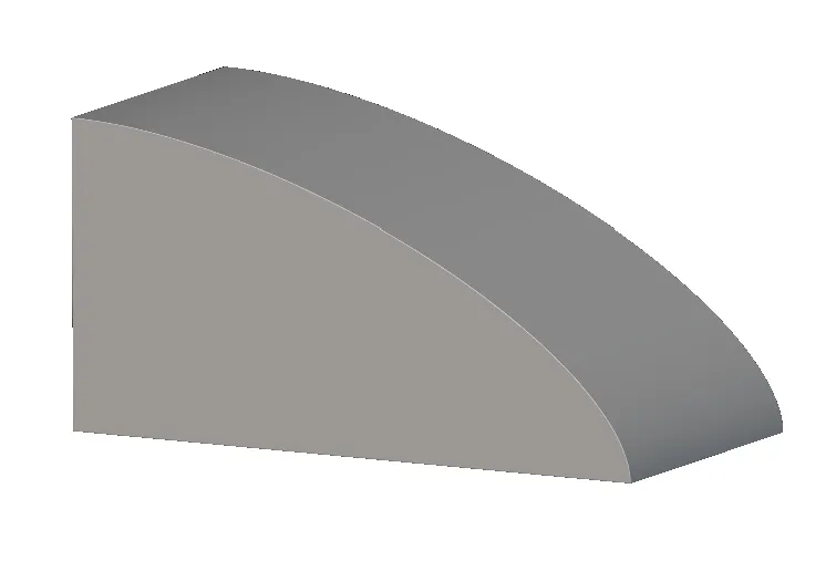
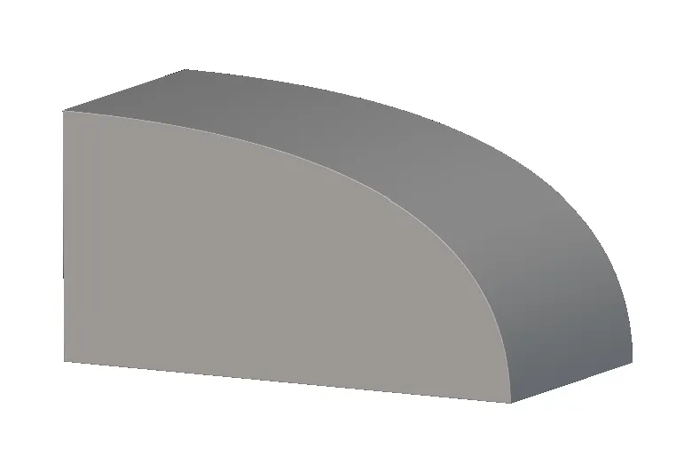
* The *Rho* Value defines the “bulge” or shape of the conic curve as it's pulled toward Point 2.
Rho Value
Resulting Curve Type
Example
Rho \< 0.5
Ellipse
Rho = 0.5
Parabola
Rho > 0.5
Hyperbola
* We have the Point 1, Point 2, and Point 3 inputs ready for the **Conic** block. The coordinate space input is the vector field representing the basis on which the curve is evaluated. For this example, it would be the XY field.
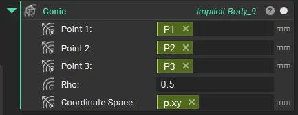
*Tip: You can also vary the value of Rho using a Ramp block.*
*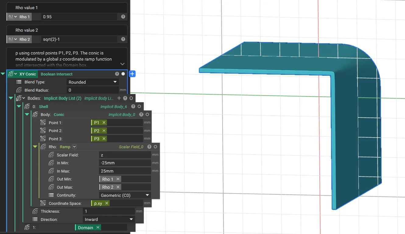*
If you want to orient the **Conic** in different directions, you can use the *Coordinate Space* input to change the direction.
### **Cubic Bézier**
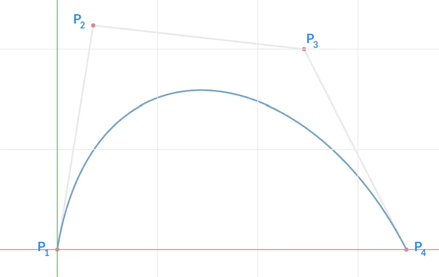
The shape of the curve is controlled by four points: Point 1 (P1), Point 2 (P2), Point 3 (P3), and Point 4 (P4).
You can vary the control points (P1−P4) for dynamic control using blocks such as a Ramp block or a Distance to Curve from Axis block.
* You will need four separate **2D Vector Field** blocks to define the inputs for **Point 1** (P1), **Point 2** (P2), **Point 3** (P3), and **Point 4** (P4).
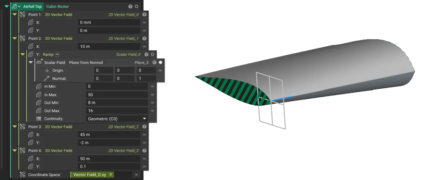
A simple example file showing how you can vary the Y coordinate of one of the points using the **Ramp** block.
## **Example File**
* [Conic Example](https://files.learn.ntop.com/Support%20Article%20Example%20Files/Knowledge%20Base/Implicit%20Modeling/conic_demo.ntop)
## Keywords:
*lofting cubic 2d wing conic bezier vector field*