> ## Documentation Index
> Fetch the complete documentation index at: https://docs.ntop.com/llms.txt
> Use this file to discover all available pages before exploring further.
# Modeling Operations
## Profile Modeling
The Profile type represents sets of coplanar curves that can be:
* open or closed
* simple or complex with multiple loops
If closed, a Profile can have multiple loops (e.g., several circles inside a rectangle). Open profiles are infinite and can be used in the same blocks as closed profiles. An open profile will automatically extend and close with lines if the infinite extensions intersect.
This flexibility enables you to create sophisticated 2D shapes that serve as the foundation for 3D geometry generation through extrusion, revolution, or sweeping operations. These operations function similarly to those in traditional CAD programs, but it's important to understand how they perform differently in nTop.
### Important Profile Field Properties
The Profile system includes two important field properties that extend its utility beyond simple 2D shape definition:
* Distance to Extrusion: is a signed distance field to the infinite extrusion relative to the profile's plane, which enables advanced geometric operations and field-driven modifications.
* Distance to Region: is an unsigned distance field to the enclosed region, which is particularly useful for creating complex internal structures or for defining simulation boundaries.
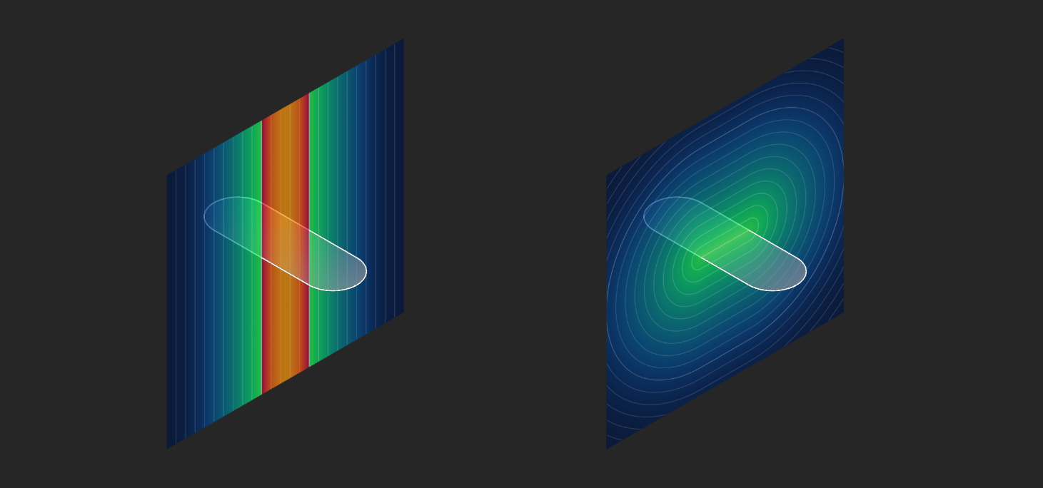 *A visual comparison between the Distance to Extrusion (left) and the Distance to Region (right) properties*
#### Using Distance to Region for Simulation Boundaries
One of the most practical applications of using the Distance to Region property is for defining boundary conditions. The example below shows an inlet boundary definition for a **Flow Analysis**.
This curved implicit body represents the fluid path for running the **Flow Analysis**. The end face that is highlighted by the red box is where we want to define the inlet boundary for the fluid.
*A visual comparison between the Distance to Extrusion (left) and the Distance to Region (right) properties*
#### Using Distance to Region for Simulation Boundaries
One of the most practical applications of using the Distance to Region property is for defining boundary conditions. The example below shows an inlet boundary definition for a **Flow Analysis**.
This curved implicit body represents the fluid path for running the **Flow Analysis**. The end face that is highlighted by the red box is where we want to define the inlet boundary for the fluid.
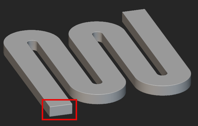 *An example fluid path for a **Flow Analysis** with the intended inlet highlighted*
Start by creating a **Plane** parallel to the surface of the intended boundary. This **Plane** is used to define the profile that matches the inlet face. The **Rectangle** profile should be almost touching the inlet surface.
*An example fluid path for a **Flow Analysis** with the intended inlet highlighted*
Start by creating a **Plane** parallel to the surface of the intended boundary. This **Plane** is used to define the profile that matches the inlet face. The **Rectangle** profile should be almost touching the inlet surface.
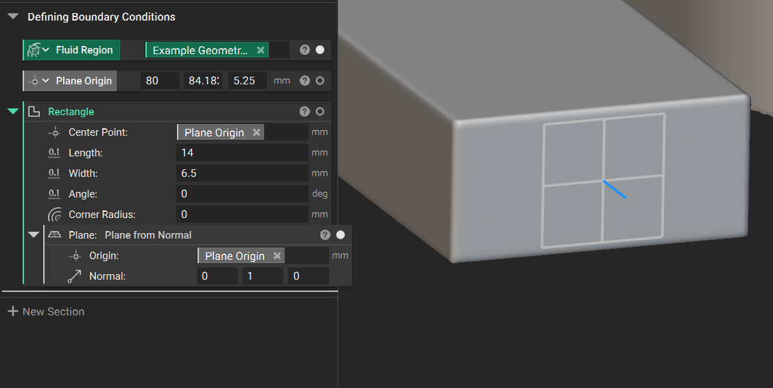 *A **Plane from Normal** created slightly offset of the inlet surface*
Extract the Distance to Region property chip from the properties panel of the **Rectangle** block. We can then use the Field Viewer to see the resulting Signed Distance Field. This field perfectly captures the area that we want to define as our inlet boundary, so we can insert the DTR variable into the *Body* input of the **Virtual Boundary by Body** block. This boundary is now capable of defining an inlet **Velocity** or **Pressure** for a **Flow Analysis**.
*A **Plane from Normal** created slightly offset of the inlet surface*
Extract the Distance to Region property chip from the properties panel of the **Rectangle** block. We can then use the Field Viewer to see the resulting Signed Distance Field. This field perfectly captures the area that we want to define as our inlet boundary, so we can insert the DTR variable into the *Body* input of the **Virtual Boundary by Body** block. This boundary is now capable of defining an inlet **Velocity** or **Pressure** for a **Flow Analysis**.
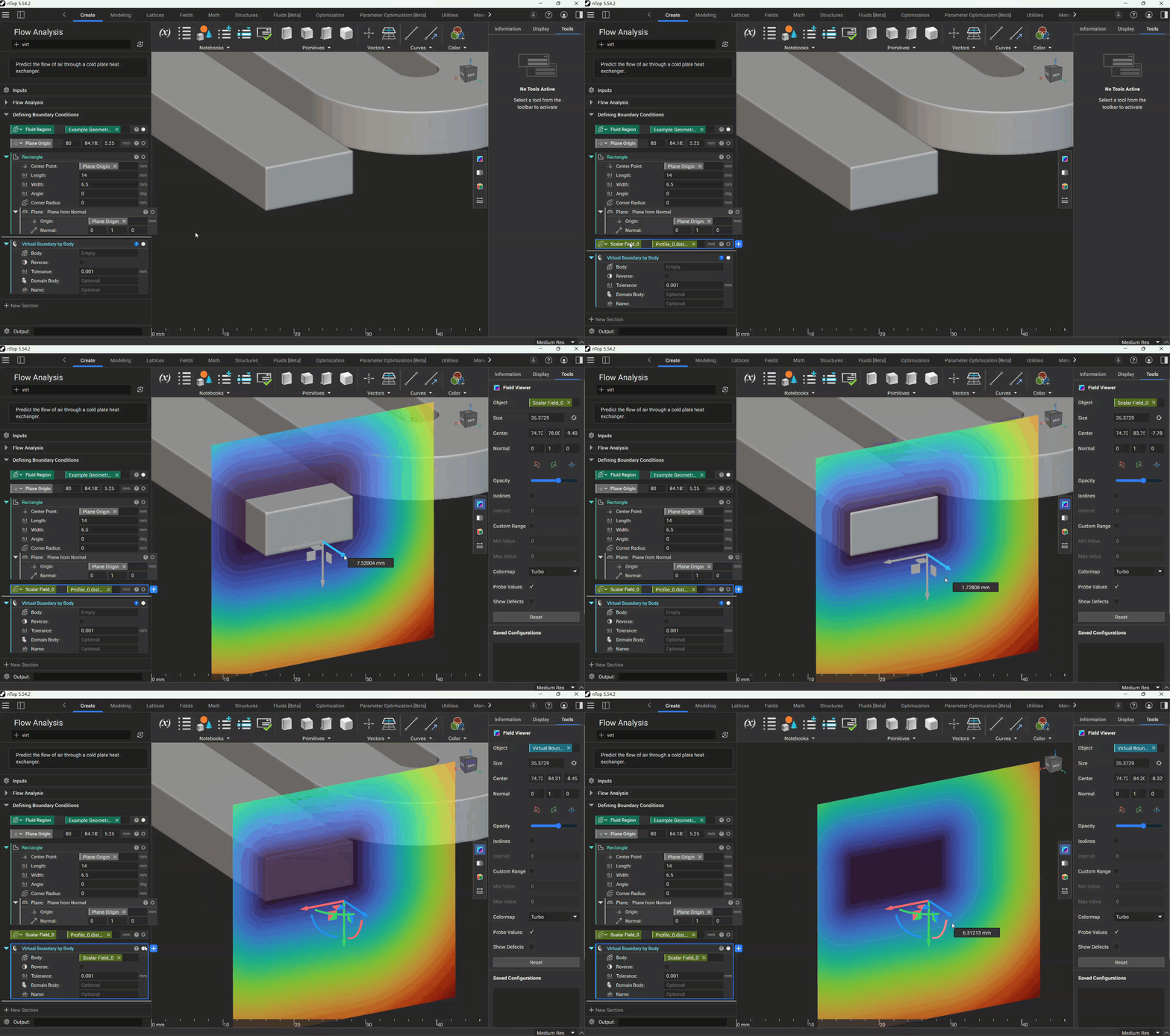 *Using the Distance to Region property of the **Rectangle** to define the inlet virtual boundary*
#### Creating Geometry using Distance to Extrusion
Considering the Distance to Extrusion property is an infinite field, we can use the **Set Bounding Box** block to visualize the geometry. This is the same concept that we learned in Lesson 1 with the infinite gyroid field example.
The example below shows a hexagon profile with its Distance to Extrusion field extracted as a variable. By placing a **Bounding Box** around a section of the infinite field, we can visualize the resulting geometry.
*Using the Distance to Region property of the **Rectangle** to define the inlet virtual boundary*
#### Creating Geometry using Distance to Extrusion
Considering the Distance to Extrusion property is an infinite field, we can use the **Set Bounding Box** block to visualize the geometry. This is the same concept that we learned in Lesson 1 with the infinite gyroid field example.
The example below shows a hexagon profile with its Distance to Extrusion field extracted as a variable. By placing a **Bounding Box** around a section of the infinite field, we can visualize the resulting geometry.
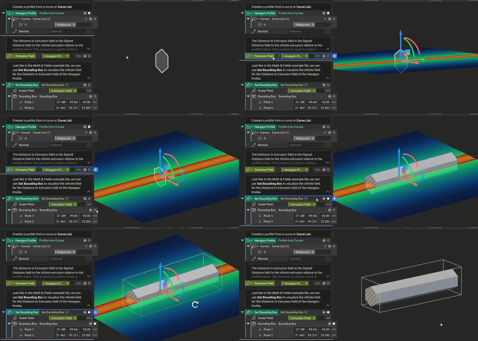 *Using a **Set Bounding Box** block on the Distance to Extrusion property of the Hexagon Profile*
Using **Set Bounding Box** in this method is only for visualizing the field geometry. The field itself is still infinite beyond the extent of the **Bounding Box**. If we were to subtract this field from a long box, the hole goes through to the other side.
*Using a **Set Bounding Box** block on the Distance to Extrusion property of the Hexagon Profile*
Using **Set Bounding Box** in this method is only for visualizing the field geometry. The field itself is still infinite beyond the extent of the **Bounding Box**. If we were to subtract this field from a long box, the hole goes through to the other side.
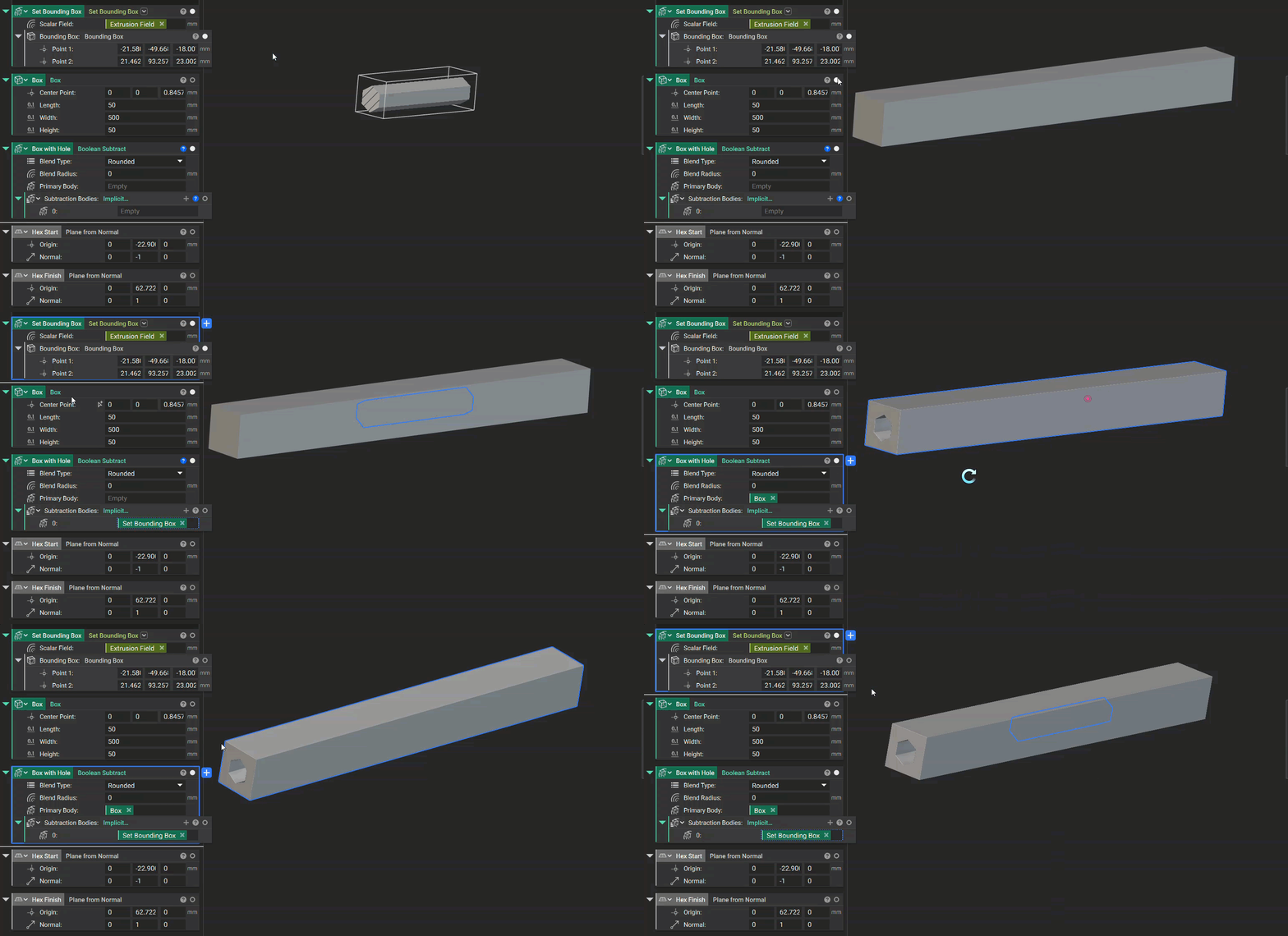 *Using **Boolean Subtract** on a **Box** to showcase the infinite hexagon field*
If we wanted to trim this infinite field and create an implicit body, the best method is to use **Boolean Intersect**. This block creates an implicit body where the geometry overlaps. In the example below, two planes are placed where we want to trim the infinite hexagon. Using **Boolean Intersect** with the two planes and the infinite field, the result is a solid implicit body, similar to performing an extrusion. If you perform this operation and the results are not as expected, check the normal direction of your planes to ensure they face away from each other, as shown below.
*Using **Boolean Subtract** on a **Box** to showcase the infinite hexagon field*
If we wanted to trim this infinite field and create an implicit body, the best method is to use **Boolean Intersect**. This block creates an implicit body where the geometry overlaps. In the example below, two planes are placed where we want to trim the infinite hexagon. Using **Boolean Intersect** with the two planes and the infinite field, the result is a solid implicit body, similar to performing an extrusion. If you perform this operation and the results are not as expected, check the normal direction of your planes to ensure they face away from each other, as shown below.
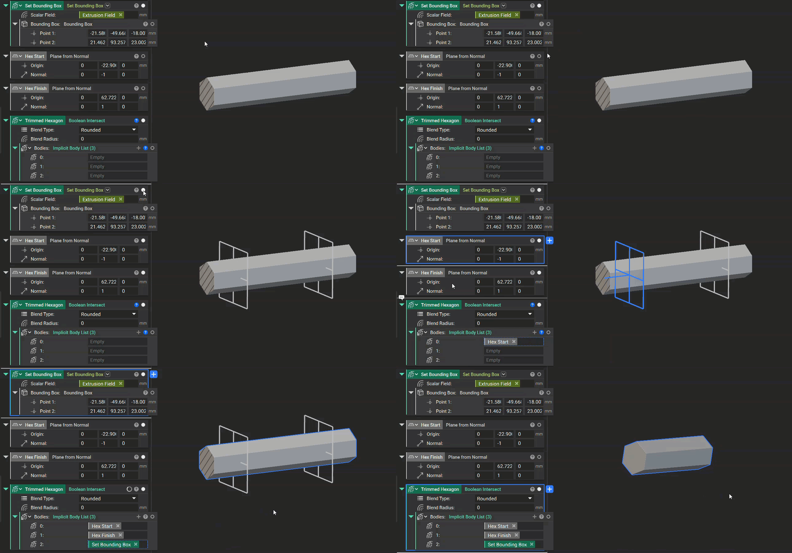 *Creating a solid body from the infinite hexagon field using **Boolean Intersect***
### “CAD Operations”
Now that we understand the underlying fields associated with profiles, we can see how these relate to native modeling blocks in nTop. In this section, we'll take a look at modeling functions that are common in traditional CAD software.
#### Extrude Profile
The **Extrude Profile** block function is essentially the same as trimming the infinite profile field. The *Distance* input defines the location of the two trimming planes, leaving only the desired implicit body between them. The *Draft Angle* input lets you taper the resulting extrusion from the starting profile to the specified distance. You can also apply the *Symmetric* bool option to create a mirrored result of the extruded profile.
*Creating a solid body from the infinite hexagon field using **Boolean Intersect***
### “CAD Operations”
Now that we understand the underlying fields associated with profiles, we can see how these relate to native modeling blocks in nTop. In this section, we'll take a look at modeling functions that are common in traditional CAD software.
#### Extrude Profile
The **Extrude Profile** block function is essentially the same as trimming the infinite profile field. The *Distance* input defines the location of the two trimming planes, leaving only the desired implicit body between them. The *Draft Angle* input lets you taper the resulting extrusion from the starting profile to the specified distance. You can also apply the *Symmetric* bool option to create a mirrored result of the extruded profile.
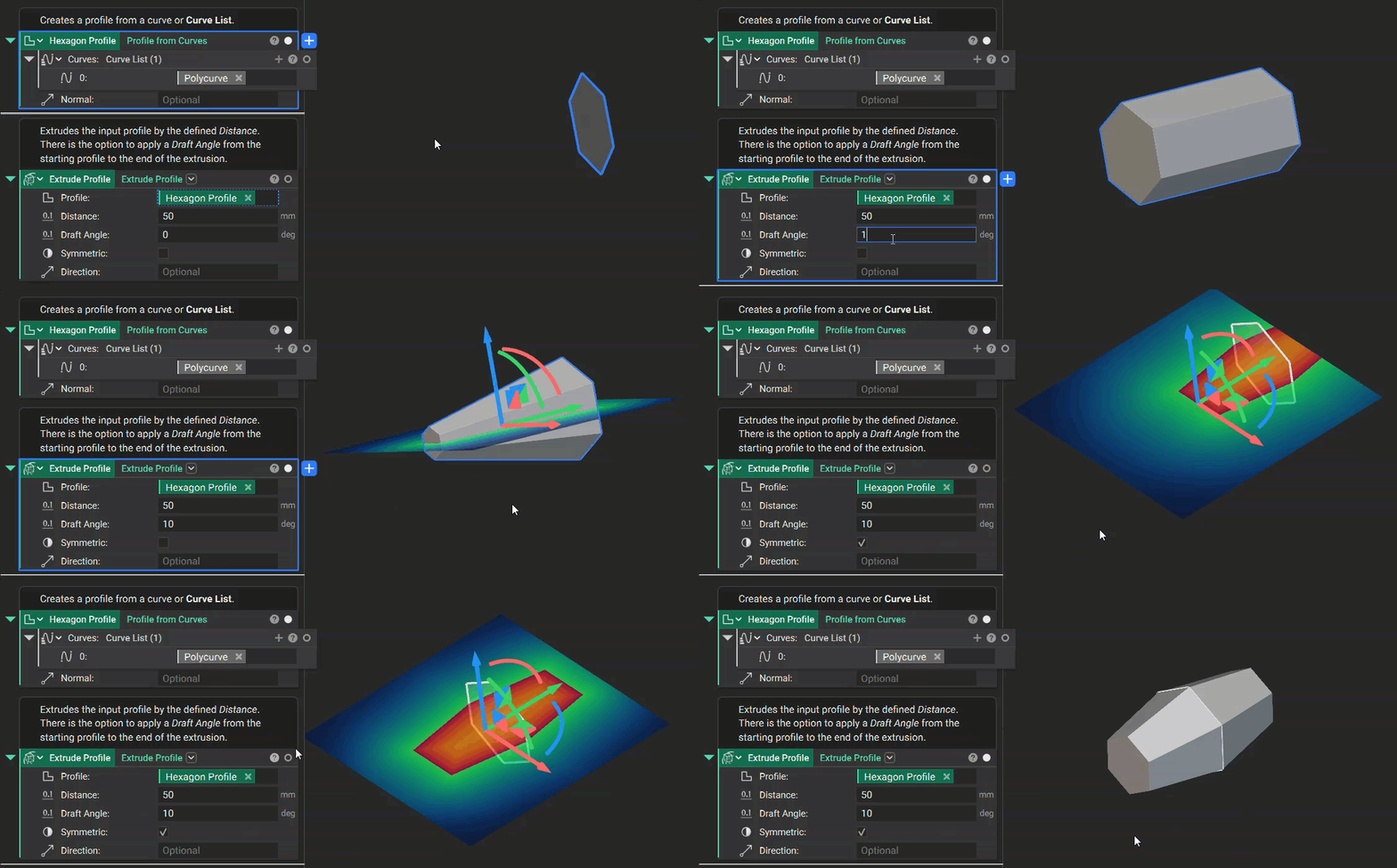 *Using the **Extrude Profile** block and demonstrating the effects of its inputs*
### Revolve Profile
The **Revolve Profile** block extrudes a profile around a specified *Axis*. The *Angle* input is similar to the *Distance* input in **Extrude Profile**, except that the distance is determined with respect to the **Axis**.
*Using the **Extrude Profile** block and demonstrating the effects of its inputs*
### Revolve Profile
The **Revolve Profile** block extrudes a profile around a specified *Axis*. The *Angle* input is similar to the *Distance* input in **Extrude Profile**, except that the distance is determined with respect to the **Axis**.
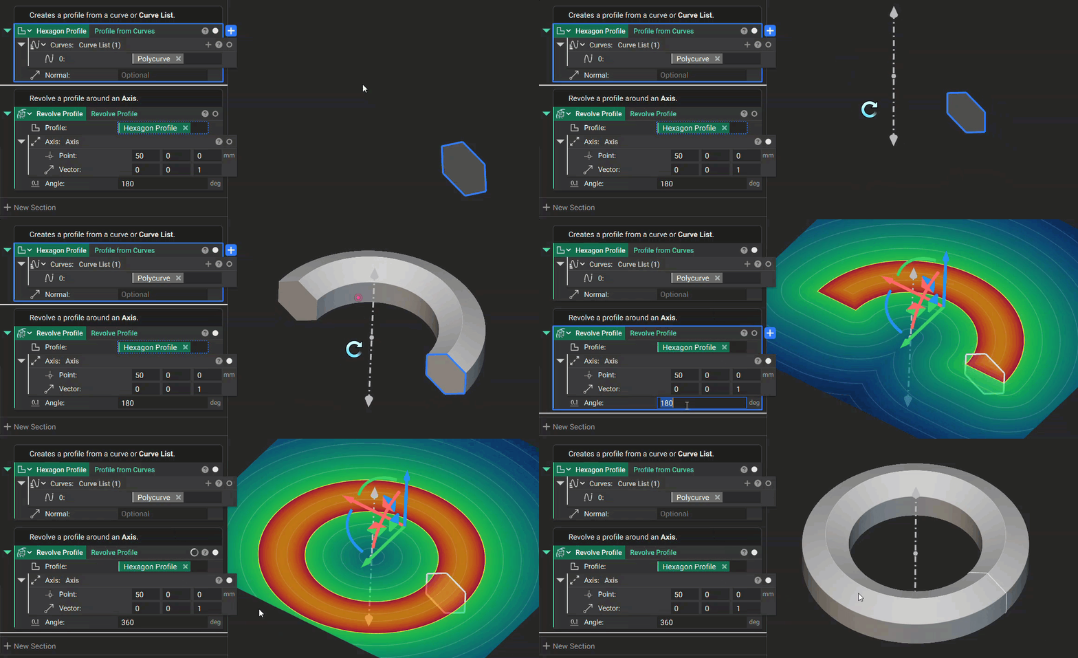 *An example of using the **Revolve Profile** block*
### Sweep Profile
The **Sweep Profile** block extrudes a *Profile* along a specified *Curve*. The *Bind Point* is the point to translate to the starting point of the *Curve*. For best results, we recommend using a *Bind Point* that is on or near the profile. The *Starting Rotation* and *Ending Rotation* inputs control the degree of rotation of the *Profile* with respect to the *Bind Point*, and to the vector tangent to the *Curve*'s starting and ending points.
You may experience longer computation times when using the **Sweep Profile** block. We are currently working on updates for our sweeping operations, users should expect performance upgrades in a future release of nTop.
*An example of using the **Revolve Profile** block*
### Sweep Profile
The **Sweep Profile** block extrudes a *Profile* along a specified *Curve*. The *Bind Point* is the point to translate to the starting point of the *Curve*. For best results, we recommend using a *Bind Point* that is on or near the profile. The *Starting Rotation* and *Ending Rotation* inputs control the degree of rotation of the *Profile* with respect to the *Bind Point*, and to the vector tangent to the *Curve*'s starting and ending points.
You may experience longer computation times when using the **Sweep Profile** block. We are currently working on updates for our sweeping operations, users should expect performance upgrades in a future release of nTop.
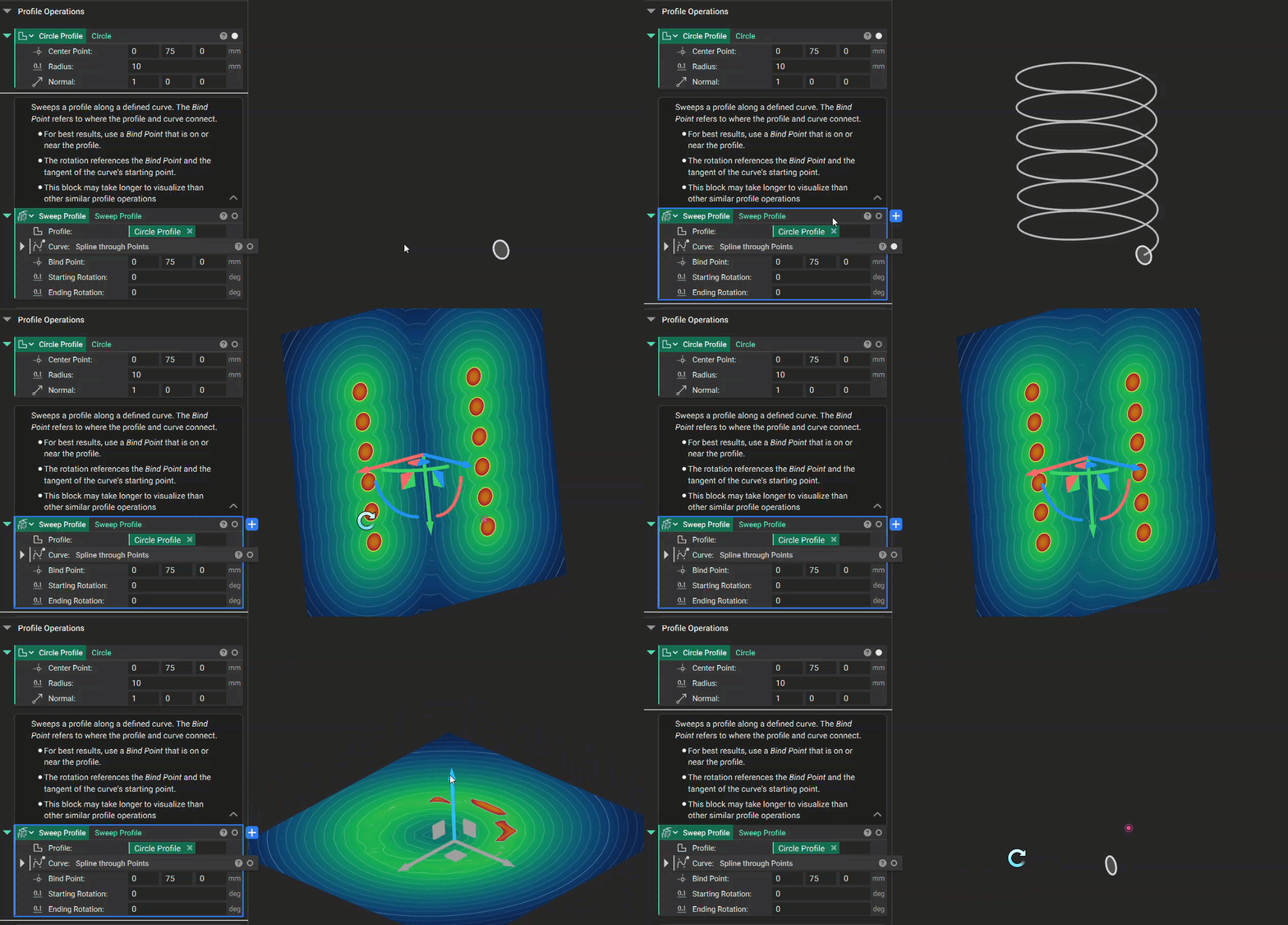 *Using **Sweep Profile** to create a spring from a **Circle** profile*
## What to Take Away:
* All Profiles have two important field properties. Knowing the difference between Distance to Extrusion and Distance to Region is important for profile modeling operations.
* **Set Bounding Box** helps with visualizing fields. Applying bounds to scalar fields helps with visualizing infinite fields.
* Profile Modeling Operations for creating implicit bodies. These blocks offer another way to create implicit bodies using profiles instead of **Boolean Intersect**.
### What's Next:
You now have an understanding of how SDFs and Profiles are connected, as well as some insight into Profile Modeling Operations.
The next lesson focuses on the opportunities of parameterizing your notebook with fields, rather than constant values.
This documentation is built and hosted on [Mintlify](https://mintlify.com), a developer documentation platform.
*Using **Sweep Profile** to create a spring from a **Circle** profile*
## What to Take Away:
* All Profiles have two important field properties. Knowing the difference between Distance to Extrusion and Distance to Region is important for profile modeling operations.
* **Set Bounding Box** helps with visualizing fields. Applying bounds to scalar fields helps with visualizing infinite fields.
* Profile Modeling Operations for creating implicit bodies. These blocks offer another way to create implicit bodies using profiles instead of **Boolean Intersect**.
### What's Next:
You now have an understanding of how SDFs and Profiles are connected, as well as some insight into Profile Modeling Operations.
The next lesson focuses on the opportunities of parameterizing your notebook with fields, rather than constant values.
This documentation is built and hosted on [Mintlify](https://mintlify.com), a developer documentation platform.