> ## Documentation Index
> Fetch the complete documentation index at: https://docs.ntop.com/llms.txt
> Use this file to discover all available pages before exploring further.
# Splines, Curves, & Profiles
## Introduction
In the previous lesson, you created implicit geometry using mathematical functions and primitives, where each shape was defined by a function evaluated throughout space. Curves are represented differently. A curve defines a path through space using exact, explicit coordinates, similar to how traditional CAD systems represent curves.
The Curves section in nTop includes many blocks for creating and modifying curves. Rather than covering every available block, this lesson focuses on several foundational curve-creation methods and demonstrates how to establish parametric relationships between them. These concepts will give you a framework to apply when working with other curve blocks.
In this lesson, you will learn why curves are represented explicitly within an implicit modeling environment and how to create fully parametric curves.
## Explicit Yet Parametric: How nTop Represents Curves
A curve also has a field. As introduced in *Course 1: Modeling with Signed Distance Fields*, every curve includes a *Scalar Field* property that represents the distance from any point in space to the nearest point on the curve. This field is useful and will be applied later in this lesson.
However, the field describes only the distance to the curve. It does not define the curve's path, including where it begins, where it ends, or how it bends. A field is evaluated at a point in space; it does not store the path itself. To define this path, nTop uses explicit coordinates, similar to a boundary representation (B-rep) CAD system.
For this reason, nTop provides several curve-creation blocks, including **Line**, **Line by Direction**, **Polyline**, **Polycurve from Curves**, **Spline by Control Points**, **Spline through Points**, and **Spline by Tangents**. Each block provides a different way to define a curve from explicit geometric information.
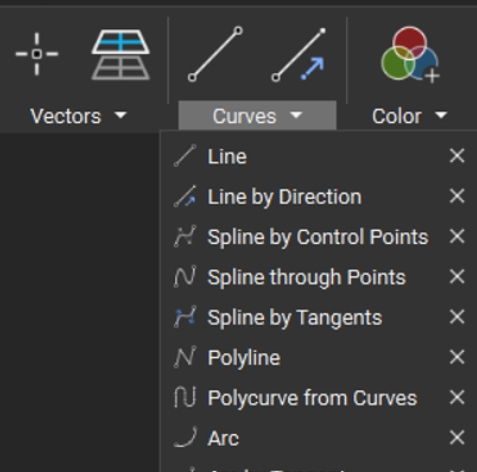 *The Curves section of the Create tab in the nTop ribbon, showing a small subset of the available curve blocks.*
Although curves are explicit, they can still be fully parametric. Their coordinates can be controlled by variables and mathematical expressions. This distinction separates explicit geometry from hard-coded geometry: a coordinate entered as a fixed value remains unchanged, while a coordinate calculated from a formula updates with the design intent.
## Building a Curve from Two Points: Line
The **Line** block creates the simplest curve in nTop. Search for the block in the Ribbon and add it to your Notebook. The block has two inputs, *Point 1* and *Point 2*, with default coordinates. Modify either point to update the line.
*The Curves section of the Create tab in the nTop ribbon, showing a small subset of the available curve blocks.*
Although curves are explicit, they can still be fully parametric. Their coordinates can be controlled by variables and mathematical expressions. This distinction separates explicit geometry from hard-coded geometry: a coordinate entered as a fixed value remains unchanged, while a coordinate calculated from a formula updates with the design intent.
## Building a Curve from Two Points: Line
The **Line** block creates the simplest curve in nTop. Search for the block in the Ribbon and add it to your Notebook. The block has two inputs, *Point 1* and *Point 2*, with default coordinates. Modify either point to update the line.
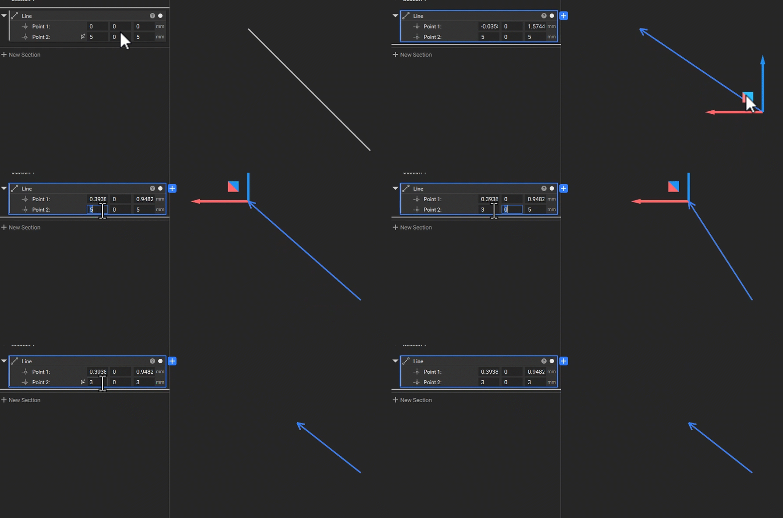 *An example of creating a **Line** in nTop*
## Parameterizing a Curve: Line by Direction
The **Line** block is useful when you know the exact coordinates of both endpoints. However, controlling the line's length or orientation through two independent points can make parameterization unnecessarily complex. For greater control, use the **Line by Direction** block.
*An example of creating a **Line** in nTop*
## Parameterizing a Curve: Line by Direction
The **Line** block is useful when you know the exact coordinates of both endpoints. However, controlling the line's length or orientation through two independent points can make parameterization unnecessarily complex. For greater control, use the **Line by Direction** block.
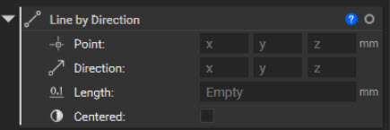 *The **Line by Direction** block*
**Line by Direction** defines a line using four inputs:
* *Point* — Defines the line's origin.
* *Direction* — Controls the line's orientation.
* *Length* — Sets the total length of the line.
* *Centered* — Determines whether the line extends from the origin in one direction or is centered about it.
Rather than requiring you to calculate a second endpoint, nTop determines it from the specified direction and length. Assigning a variable to Length lets you control the line elsewhere in the Notebook, establishing the parametric relationship used in the next section.
## Encoding Design Intent with Trigonometry
You don't need to define explicit geometry with manually entered coordinates. A curve remains explicit when its points are calculated from formulas; its coordinates simply update as the formula inputs change. Trigonometry provides a direct way to encode this behavior by converting an angle and a known length into precise dimensions.
### Creating a Right Triangle from One Angle and One Length
Now we will create a right triangle controlled by two variables: the length of its hypotenuse and the angle between the hypotenuse and the X axis. If you parameterize it correctly, the adjacent and opposite leg lengths will update automatically.
1. Add a **Line by Direction** block.
2. Set *Point* to the *Origin* variable at *(0, 0, 0)*.
3. Set *Direction* to *(1, 0, 0)* to align the line with the X axis.
4. Create a variable named *Hypotenuse Length* and set its value to *120 mm*. Assign this variable to the line's *Length* input.
*The **Line by Direction** block*
**Line by Direction** defines a line using four inputs:
* *Point* — Defines the line's origin.
* *Direction* — Controls the line's orientation.
* *Length* — Sets the total length of the line.
* *Centered* — Determines whether the line extends from the origin in one direction or is centered about it.
Rather than requiring you to calculate a second endpoint, nTop determines it from the specified direction and length. Assigning a variable to Length lets you control the line elsewhere in the Notebook, establishing the parametric relationship used in the next section.
## Encoding Design Intent with Trigonometry
You don't need to define explicit geometry with manually entered coordinates. A curve remains explicit when its points are calculated from formulas; its coordinates simply update as the formula inputs change. Trigonometry provides a direct way to encode this behavior by converting an angle and a known length into precise dimensions.
### Creating a Right Triangle from One Angle and One Length
Now we will create a right triangle controlled by two variables: the length of its hypotenuse and the angle between the hypotenuse and the X axis. If you parameterize it correctly, the adjacent and opposite leg lengths will update automatically.
1. Add a **Line by Direction** block.
2. Set *Point* to the *Origin* variable at *(0, 0, 0)*.
3. Set *Direction* to *(1, 0, 0)* to align the line with the X axis.
4. Create a variable named *Hypotenuse Length* and set its value to *120 mm*. Assign this variable to the line's *Length* input.
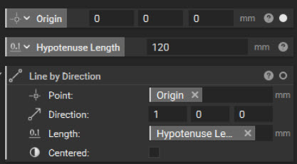 *The **Line by Direction** block utilizing the Origin and Hypotenuse Length variables for its inputs*
5. Add a **Rotate Object** block, drag your created **Line by Direction** block to its *Object* input, and make the block a variable named *Hypotenuse*.
6. Set *Rotation Center* to the *Origin* variable.
7. Set *Axis* to *(0, 0, 1)* to rotate the line about the Z axis.
8. Create a variable named *Hypotenuse Angle* and set its value to *35 deg*. Assign this variable to the *Angle* input.
*The **Line by Direction** block utilizing the Origin and Hypotenuse Length variables for its inputs*
5. Add a **Rotate Object** block, drag your created **Line by Direction** block to its *Object* input, and make the block a variable named *Hypotenuse*.
6. Set *Rotation Center* to the *Origin* variable.
7. Set *Axis* to *(0, 0, 1)* to rotate the line about the Z axis.
8. Create a variable named *Hypotenuse Angle* and set its value to *35 deg*. Assign this variable to the *Angle* input.
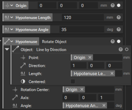 *Creating the Hypotenuse by rotating the original line*
The resulting line represents the triangle's hypotenuse. You can now control its length and angle independently through the two variables.
That single angle now determines the whole triangle. Using SOH-CAH-TOA:
* *Adjacent leg length* = *hypotenuse length* × Cos(*hypotenuse angle*)
* *Opposite leg length* = *hypotenuse length* × *Sin*(*hypotenuse angle*)
We can build the *Adjacent leg length* and *Opposite leg length* using the math blocks:
*Creating the Hypotenuse by rotating the original line*
The resulting line represents the triangle's hypotenuse. You can now control its length and angle independently through the two variables.
That single angle now determines the whole triangle. Using SOH-CAH-TOA:
* *Adjacent leg length* = *hypotenuse length* × Cos(*hypotenuse angle*)
* *Opposite leg length* = *hypotenuse length* × *Sin*(*hypotenuse angle*)
We can build the *Adjacent leg length* and *Opposite leg length* using the math blocks:
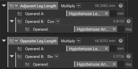 *Calculating the lengths of the legs using trigonometry*
Now let's create the Adjacent and Opposite Legs:
1. Add a **Line by Direction** block and make it a variable named the *Adjacent Leg.*
2. Set *Point* to the *Start Point* property of the *Hypotenuse*.
3. Set *Direction* to *(1, 0, 0)*.
4. Set *Length* to the calculated *Adjacent Leg Length*.
*Calculating the lengths of the legs using trigonometry*
Now let's create the Adjacent and Opposite Legs:
1. Add a **Line by Direction** block and make it a variable named the *Adjacent Leg.*
2. Set *Point* to the *Start Point* property of the *Hypotenuse*.
3. Set *Direction* to *(1, 0, 0)*.
4. Set *Length* to the calculated *Adjacent Leg Length*.
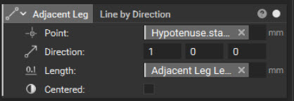 *Defining the Adjacent Leg using the new length calculation*
5. Add another **Line by Direction** block and make it a variable named the Opposite Leg.
6. Set *Point* to the adjacent leg's *End Point* property.
7. Set *Direction* to *(0, 1, 0)*.
8. Set *Length* to the calculated *Opposite Leg Length*.
*Defining the Adjacent Leg using the new length calculation*
5. Add another **Line by Direction** block and make it a variable named the Opposite Leg.
6. Set *Point* to the adjacent leg's *End Point* property.
7. Set *Direction* to *(0, 1, 0)*.
8. Set *Length* to the calculated *Opposite Leg Length*.
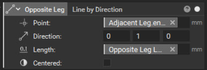 *Defining the Opposite Leg using the new length calculation*
Because these lines reference property chips instead of manually entered coordinates, their endpoints remain connected when the *Hypotenuse Length* or *Hypotenuse Angle* changes.
Now we can combine the segments into a closed curve:
1. Add a **Polycurve from Curves** block.
2. Add the following curves to its list:
* *Adjacent Leg*
* *Opposite Leg*
* *Hypotenuse*
*Defining the Opposite Leg using the new length calculation*
Because these lines reference property chips instead of manually entered coordinates, their endpoints remain connected when the *Hypotenuse Length* or *Hypotenuse Angle* changes.
Now we can combine the segments into a closed curve:
1. Add a **Polycurve from Curves** block.
2. Add the following curves to its list:
* *Adjacent Leg*
* *Opposite Leg*
* *Hypotenuse*
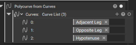 *Creating the polycurve using the legs and Hypotenuse*
The **Polycurve from Curves** block requires consecutive curves to share endpoints and reports an error if the segments don't align.
Finally, change the *Hypotenuse Angle* from *35°* to *60°*. The triangle reshapes automatically while preserving the relationships encoded in the workflow.
*Creating the polycurve using the legs and Hypotenuse*
The **Polycurve from Curves** block requires consecutive curves to share endpoints and reports an error if the segments don't align.
Finally, change the *Hypotenuse Angle* from *35°* to *60°*. The triangle reshapes automatically while preserving the relationships encoded in the workflow.
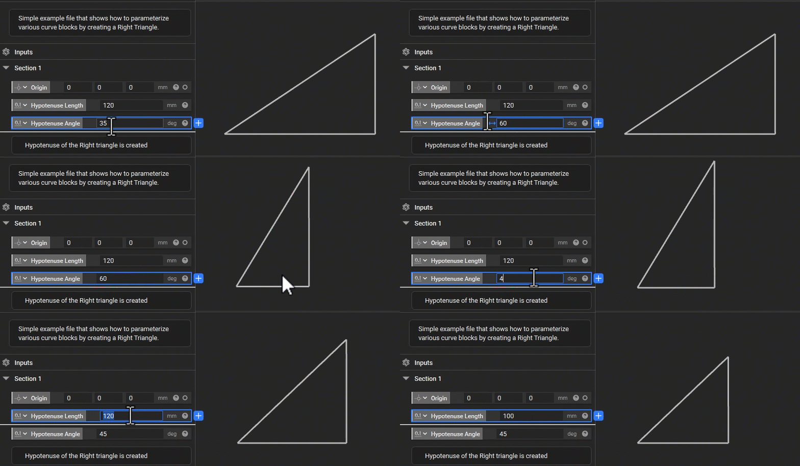 *Adjusting the Hypotenuse Angle or Length variables cause the triangle to recalculate and rebuild*
For the completed workflow, you can download the following nTop File:
**Downloadable Files:**
[Example File Download](https://files.learn.ntop.com/Courses/nTop%20Foundational%20Learning%20Course/Course%202/nTop%20Files/C2S1_Lesson2_MakingRightTriangle.ntop)
*This file was last updated in nTop 6.03*
### An Equivalent Approach: Polyline from Explicit Points
You can create the same triangle with a **Polyline** block. Instead of constructing three individual line segments, this approach calculates the triangle's vertices and connects them in sequence.
Using the same variables and trigonometric relationships, define the vertices as follows by creating three **Point** blocks using the coordinates below. Use math expressions to calculate the required X and Y components.
* **Point 1:** *(0, 0, 0)*
*Adjusting the Hypotenuse Angle or Length variables cause the triangle to recalculate and rebuild*
For the completed workflow, you can download the following nTop File:
**Downloadable Files:**
[Example File Download](https://files.learn.ntop.com/Courses/nTop%20Foundational%20Learning%20Course/Course%202/nTop%20Files/C2S1_Lesson2_MakingRightTriangle.ntop)
*This file was last updated in nTop 6.03*
### An Equivalent Approach: Polyline from Explicit Points
You can create the same triangle with a **Polyline** block. Instead of constructing three individual line segments, this approach calculates the triangle's vertices and connects them in sequence.
Using the same variables and trigonometric relationships, define the vertices as follows by creating three **Point** blocks using the coordinates below. Use math expressions to calculate the required X and Y components.
* **Point 1:** *(0, 0, 0)*
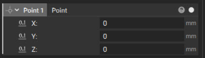 *A **Point** block located at the origin*
* **Point 2:** *(Hypotenuse Length × Cos(Hypotenuse Angle), 0, 0)*
*A **Point** block located at the origin*
* **Point 2:** *(Hypotenuse Length × Cos(Hypotenuse Angle), 0, 0)*
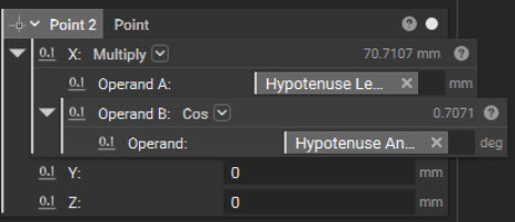 *Calculating the Point 2 X location using trigonometry*
* **Point 3:** *(Hypotenuse Length × Cos(Hypotenuse Angle), Hypotenuse Length × Sin(Hypotenuse Angle), 0)*
*Calculating the Point 2 X location using trigonometry*
* **Point 3:** *(Hypotenuse Length × Cos(Hypotenuse Angle), Hypotenuse Length × Sin(Hypotenuse Angle), 0)*
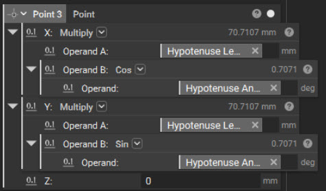 *Calculating the Point 3 X and Y locations using trigonometry*
To construct the triangle:
1. Add a **Polyline** block.
2. Add the points to its list in the following order:
* *Point 1*
* *Point 2*
* *Point 3*
* *Point 1*
3. Repeat *Point 1* as the final entry to close the triangle.
*Calculating the Point 3 X and Y locations using trigonometry*
To construct the triangle:
1. Add a **Polyline** block.
2. Add the points to its list in the following order:
* *Point 1*
* *Point 2*
* *Point 3*
* *Point 1*
3. Repeat *Point 1* as the final entry to close the triangle.
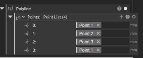 *Building the **Polyline** using the newly calculated points*
The **Polyline** block connects each consecutive pair of points with a straight segment. Therefore, the point order determines the resulting shape.
Both approaches produce the same parameterized triangle. **Polycurve from Curves** is generally more appropriate when the design consists of separate, reusable curve segments. **Polyline** is more direct when the design intent is defined by an ordered collection of positions.
To create a profile from these curves, use the **Profile from Curves** block.
*Building the **Polyline** using the newly calculated points*
The **Polyline** block connects each consecutive pair of points with a straight segment. Therefore, the point order determines the resulting shape.
Both approaches produce the same parameterized triangle. **Polycurve from Curves** is generally more appropriate when the design consists of separate, reusable curve segments. **Polyline** is more direct when the design intent is defined by an ordered collection of positions.
To create a profile from these curves, use the **Profile from Curves** block.
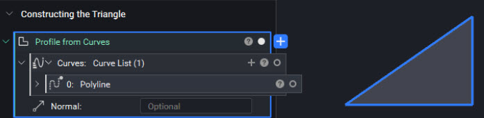 *Creating the triangle profile using the **Profile from Curves** block and the **Polyline***
The resulting profile provides the foundation for generating 3D geometry from a 2D sketch. In the next lesson, you will explore profile creation in greater depth and learn how to use profiles with operations such as **Extrude**, **Revolve**, and **Sweep**.
For the completed workflow, you can download the following nTop File:
**Downloadable Files:**
[Example File Download](https://files.learn.ntop.com/Courses/nTop%20Foundational%20Learning%20Course/Course%202/nTop%20Files/C2S1_Lesson2_MakingRightTrianglePoints.ntop)
*This file was last updated in nTop 6.03*
## What to Take Away
* Curves are represented by explicit coordinates that define their path through space, even though each curve also provides a *Scalar Field* representing distance to the curve.
* Explicit geometry can still be fully parametric when coordinates, dimensions, and orientations are controlled by variables, expressions, and referenced properties.
* Mathematical relationships, including trigonometric expressions, allow related curve dimensions to update automatically while preserving design intent.
* Referencing curve properties, such as *Start Point* and *End Point*, keeps connected geometry aligned as input parameters change.
* Use **Polycurve from Curves** to combine separate curve segments and **Polyline** to connect an ordered sequence of points.
* Closed curves can be converted into profiles with **Profile from Curves**, providing the foundation for 3D operations such as **Extrude**, **Revolve**, and **Sweep**.
## What's Next
You now understand how to create parametric curves in nTop. In the next lesson, you will learn how to create profiles and use them with common operations such as **Extrude**, **Revolve**, and **Sweep**.
This documentation is built and hosted on [Mintlify](https://mintlify.com), a developer documentation platform.
*Creating the triangle profile using the **Profile from Curves** block and the **Polyline***
The resulting profile provides the foundation for generating 3D geometry from a 2D sketch. In the next lesson, you will explore profile creation in greater depth and learn how to use profiles with operations such as **Extrude**, **Revolve**, and **Sweep**.
For the completed workflow, you can download the following nTop File:
**Downloadable Files:**
[Example File Download](https://files.learn.ntop.com/Courses/nTop%20Foundational%20Learning%20Course/Course%202/nTop%20Files/C2S1_Lesson2_MakingRightTrianglePoints.ntop)
*This file was last updated in nTop 6.03*
## What to Take Away
* Curves are represented by explicit coordinates that define their path through space, even though each curve also provides a *Scalar Field* representing distance to the curve.
* Explicit geometry can still be fully parametric when coordinates, dimensions, and orientations are controlled by variables, expressions, and referenced properties.
* Mathematical relationships, including trigonometric expressions, allow related curve dimensions to update automatically while preserving design intent.
* Referencing curve properties, such as *Start Point* and *End Point*, keeps connected geometry aligned as input parameters change.
* Use **Polycurve from Curves** to combine separate curve segments and **Polyline** to connect an ordered sequence of points.
* Closed curves can be converted into profiles with **Profile from Curves**, providing the foundation for 3D operations such as **Extrude**, **Revolve**, and **Sweep**.
## What's Next
You now understand how to create parametric curves in nTop. In the next lesson, you will learn how to create profiles and use them with common operations such as **Extrude**, **Revolve**, and **Sweep**.
This documentation is built and hosted on [Mintlify](https://mintlify.com), a developer documentation platform.