About this Block
What it does: The Parameter Optimization block performs an optimization algorithm to find the collection of optimal design parameters. It works by iteratively adjusting a set of Design Parameters to either minimize or maximize a defined Objective while satisfying all specified Constraints.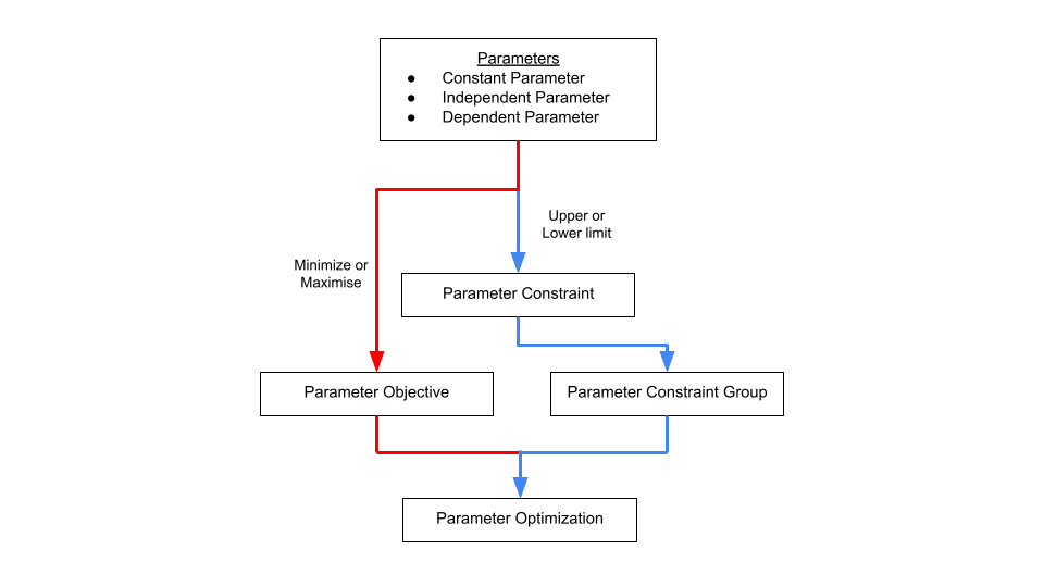 Common uses:
- Finding the lightest possible design that meets all structural requirements.
- Maximizing a component’s stiffness while keeping its mass below a certain limit.
- Optimizing a part’s geometry to improve its performance under various conditions.
- The Constraints and Tracked Parameters inputs are optional.
- Use Constraints to set limits on your design.
- Use Tracked Parameters to monitor additional variables during the optimization run for debugging or detailed analysis.
- The Algorithm input determines the specific method used to find the optimal solution.
Grid
- This method performs uniform grid sampling. It performs an exhaustive search by evaluating every possible combination of parameter values on a predefined grid. You specify the total number of “steps” for each variable, and the optimizer tests them all.
- This algorithm is Ideal for understanding the design space before using an additional optimization algorithm.
| | |
| --- | --- |
|
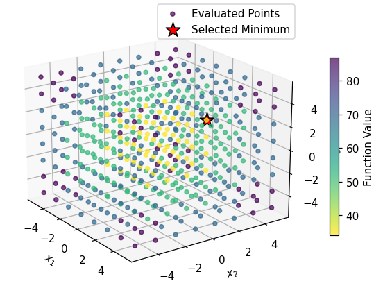 | What you see: A perfect 3D cube of points. The algorithm tests every single point on this predefined grid. The final result (the red star) is simply the point on the grid that had the lowest value in the case of a minimization problem.
Takeaway: This method is simple and exhaustive, but scales terribly. For our 3D problem with 8 values per axis, it ran 8^3 = 512 calculations. For a 10D problem, it would be 8^10 (over 1 billion), making it completely impractical for some real-world problems. It will also miss the true minimum if it falls between the grid points.|
Global
- This method uses a global optimization algorithm. It is a sophisticated method that splits its effort between exploring new, untested regions of the design space (exploration) and performing local optimization on promising regions (exploitation).
- This algorithm is suitable for finding a global maximum/minimum among multiple local maximums or minimums.
| | |
| --- | --- |
|
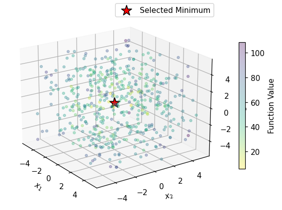 | What you see: A large “cloud” of points scattered across the entire 3D space, with a mix of colors. This shows the algorithm is actively exploring new, random regions. The final red star is correctly placed at the true global minimum (0,0,0).
Takeaway: This algorithm is designed to solve difficult problems. It intelligently balances exploration (sampling new regions to find the best valley) with exploitation (using local search to find the bottom of that valley). It is highly effective at avoiding local traps and finding the true global minimum.|
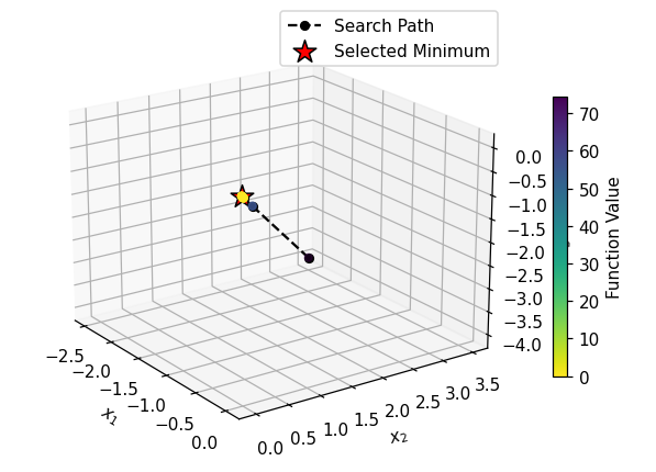
Local
- This method uses a local BOBYQA technique. BOBYQA (Bound Optimization BY Quadratic Approximation) builds a smooth, quadratic approximation of your objective function within the local region of your current solution and seeks the minimum of that approximation.
- This algorithm is suitable when you are looking for a minimum/maximum of a simple convex/concave optimization problem.
| | |
| --- | --- |
|
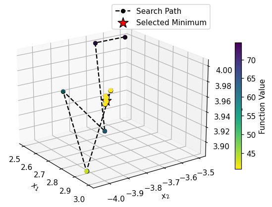 | What you see: A black search path starting from its initial guess. The algorithm intelligently creates a smooth model of the “valley” it’s in and follows it downhill to the bottom. The final red star is at a local minimum, but not the true global one at (0,0,0).
Takeaway: This is a powerful and efficient local optimizer that doesn’t require gradients and can handle a certain level of noise or non-smoothness in functions. However, it is entirely dependent on its starting point and has no way to escape the first valley it finds.|
Smooth
- This method is a Gradient-Based (LBFGS) optimization. It uses a finite difference approximation to calculate the gradients of your objective function and then follows these gradients to find a minimum.
-
This algorithm is best used when your dependent parameters are smooth and continuous.
| | |
| --- | --- |
|
 | What you see: A short, efficient black search path. The algorithm uses the function’s slope (gradient) to find the steepest path downhill from its starting point. Like BOBYQA, it quickly finds the bottom of the nearest valley and gets stuck there.
Takeaway: This method performs very well and is the standard for “smooth” problems (common in machine learning). It may scale poorly, however, when dealing with too many parameters due to the finite difference computation for gradients. In addition, its reliance on the local gradient makes it blind to the bigger picture, and it will get trapped in the first local minimum it encounters.| - The Max Iterations input sets a limit on the number of attempts the block will make to find a solution, preventing excessively long run times.
- We recommend performing a Global or Grid search first to identify parameters that can be used to with the Local algorithm.
Example File
Download Example: Parameter Optimization
Runs an optimization algorithm to find the collection of Design Parameters that produce an optimal Parameter Objective value while satisfying all Parameter Constraints.
Inputs
| Name | Type | Description |
|---|---|---|
| Objective | Parameter Objective | The objective function for the optimization process. |
| Constraints | Parameter Constraint Group | The constraints to satisfy during the optimization process. |
| Design parameters | Parameter Group | The collection of Parameters the algorithm will change in its search for the optimal solution. |
| Algorithm | Optimization Algorithm Enum | The specific optimization method to be used. This dictates how the block will search for the optimal solution. |
| Max iterations | Integer | The maximum number of iterations allowed during the optimization process. |
| Tracked parameters | Parameter Group | Additional Parameters to be tracked and logged during the optimization process. Useful for debugging or detailed analysis. |