Aircraft Flow Analysis

Fluids [Beta]/Analysis/aircraft_flow_analysis

​

About this Block

What it does: The Aircraft Analysis block calculates time-averaged and instantaneous pressure, velocity, and boundary force fields around aircraft geometries using the Lattice Boltzmann Method (LBM). It uses a solver setup optimized for external aerodynamics, producing results specialized for lifting bodies and surfaces that differ from the standard Flow Analysis block Note: This block requires an NVIDIA GPU Common uses:

• Predicting lift and drag coefficients across a range of angles of attack.
• Analyzing surface pressure distributions and identifying flow separation zones.
• Comparing aerodynamic performance between geometry variants or configurations.
• Capturing unsteady wake structures and vortex shedding behind lifting surfaces.

Setup Requirements: Ensure the following conditions are met before running the block:

• The geometry must be a closed, watertight surface representing the aircraft.
• No manual fluid domain or far-field boundary conditions are required; the block generates these automatically.

Automated Simulation Setup: The block automatically constructs a simulation domain by extending the geometry’s bounding box. The resulting domain length can be calculated using the formula L_i(pad) ≈ L_i × (1 + p_i⁻ + p_i⁺), using the following padding factors p_i:

​

Simulation Domain Padding Example

The padded domain length is estimated as: L_i(pad) ≈ L_i × (1 + p_i⁻ + p_i⁺) where L_i is the bounding box span in direction i, and p_i⁻, p_i⁺ are the upstream/downstream padding factors.

​

Reference Geometry: Aircraft Flow Analysis

Bounding box spans L_i: Example — X axis: L_x(pad) ≈ 18,615.74 × (1 + 0.5 + 1.5) = 18,615.74 × 3.0 = 55,847.22 mm Example — Z axis: L_z(pad) ≈ 3,738.44 × (1 + 1.5 + 1.0) = 3,738.44 × 3.5 = 13,084.54 mm

• Boundary Conditions: The upstream face applies a velocity inlet, while the downstream face applies a pressure outlet. Lateral far-field faces use a slip boundary condition to minimize wall interference.
• Surface Modeling: A wall model is applied automatically to the aircraft surface.
• Compressibility: For higher Mach numbers, a Prandtl-Glauert compressibility correction is applied. Note that as the Mach number approaches 0.7, this correction noticeably reduces effective resolution in the Y and Z directions; plan your Cell Size accordingly.

Tips on Cell Size: The simulation uses a uniform Cartesian mesh defined by the Cell Size parameter.

• Quantitative Results: To achieve accurate force coefficients, resolve the smallest relevant features (e.g., gaps, control surface edges, or slat tracks) with at least 7 cells.
• Qualitative Results: For flow visualization and identifying separation patterns, a minimum of 3 cells across the smallest feature is sufficient.
• Memory Estimation: Ten million cells require approximately 1.3 GB of dedicated GPU memory. This is roughly 30% higher than the Flow Analysis block due to force field computations.

​

Memory Estimate

Given a uniform cell size of Δ = 330 mm, the approximate cell count per axis is: N_i = ⌈ L_i(pad) / Δ ⌉ Total cell count: N_total = N_x × N_y × N_z = 169 × 101 × 40 ≈ 682,360 cells Estimated GPU memory using the reference rate of 1.3 GB per 10 million cells: M ≈ (682,360 / 10,000,000) × 1.3 GB ≈ 88.7 MB Notes on Transient Simulations:

• Iterative Process: LBM is inherently transient and advances the solution through discrete time steps until results are statistically steady-state.
• Instantaneous vs. Time-Averaged: The block exposes two result fields. The instantaneous field (first) captures unsteady fluctuations like turbulence and vortex dynamics. The time-averaged field (second) reveals the mean flow structure suitable for coefficient extraction.
• Force Coefficients: Lift, drag, and moment coefficients are derived from the time-averaged boundary force field as the simulation converges.

How to Use and Analyze Results:

1. Run the Simulation: Run the block. The simulation advances until it reaches a steady state and outputs a CFD Analysis Result, which is used for visualization and data extraction.
2. View Streamlines: To visualize the flow field, select the result in the notebook and update its Display Mode to Streamlines in the View Settings.
3. Extract Near-Body Data (Advanced): To extract data points from a specific area (e.g., near the aircraft surface):
   • Find Region ID: Select the block and switch the Heads-Up Display (HUD) to Cell Region. Identify the region ID you want to analyze (e.g., Region 3 is typically the area near the body).
   • Filter Points: Add a Filter Cell Region block. Input the CFD Analysis Result and the Region ID to generate a Point List.
   • Evaluate Data: Use the Evaluate Field block with the Point List for detailed analysis of pressure or velocity near the surface.

Tips for Resolving Errors:

• Solver Diverged: Verify that the Mach number and angle of attack are within supported ranges. Ensure the Cell Size is not too coarse; poorly resolved gaps or excessively large time steps are common causes.
• Geometry Issues: Ensure the surface is watertight and free of self-intersections or open edges. Non-manifold geometry causes incorrect wall detection.
• Insufficient GPU Memory: Incrementally increase the Cell Size or simplify the geometry to remove small features that drive up cell count without impacting the primary aerodynamic result.
• Incorrect far-field domain: The simulation domain is derived from the geometry’s bounding box, which can sometimes be computed incorrectly for certain complex implicits. If the domain looks wrong, use a Voxel Grid From Implicit block to voxelize the geometry, convert it back to an implicit, and set the bounding box of the original geometry to that explicitly.

​

Example File

Download Example: Aircraft Flow Analysis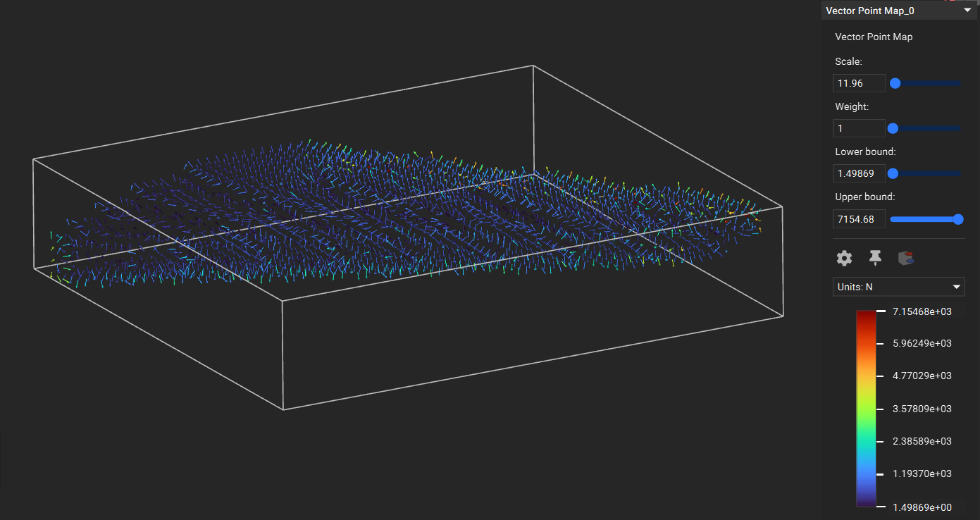

---

Calculates the pressure, velocity, and surface forces on an implicit body. The implicit body must be oriented in the default aircraft position with flow direction aligned to the positive X-axis, Y-axis the starboard/right wing direction and Z-axis pointing upward (lift direction). The solution uses a Lattice Boltzmann Method. A transient simulation is initiated and continues until the flow reaches a statistically steady state, then returns time-averaged pressure, velocity fields, along with the force on the implicit body surfaces. Streamlines will be calculated on the time-averaged velocity results. This block requires an NVIDIA GPU.

​

Inputs

​

Outputs