Objective:
Learn how to set up and run a Conjugate Heat Transfer (CHT) analysis in nTop. This feature extends the standard Flow Analysis by coupling fluid flow with solid heat conduction. In this guide, we will use a Heat Sink example to demonstrate how to simulate cooling performance by analyzing the interaction between an airflow channel and a solid aluminum heat sink.Applies to:
- nTop 5.38 or later (requires nTop Fluids capabilities).
Procedure:
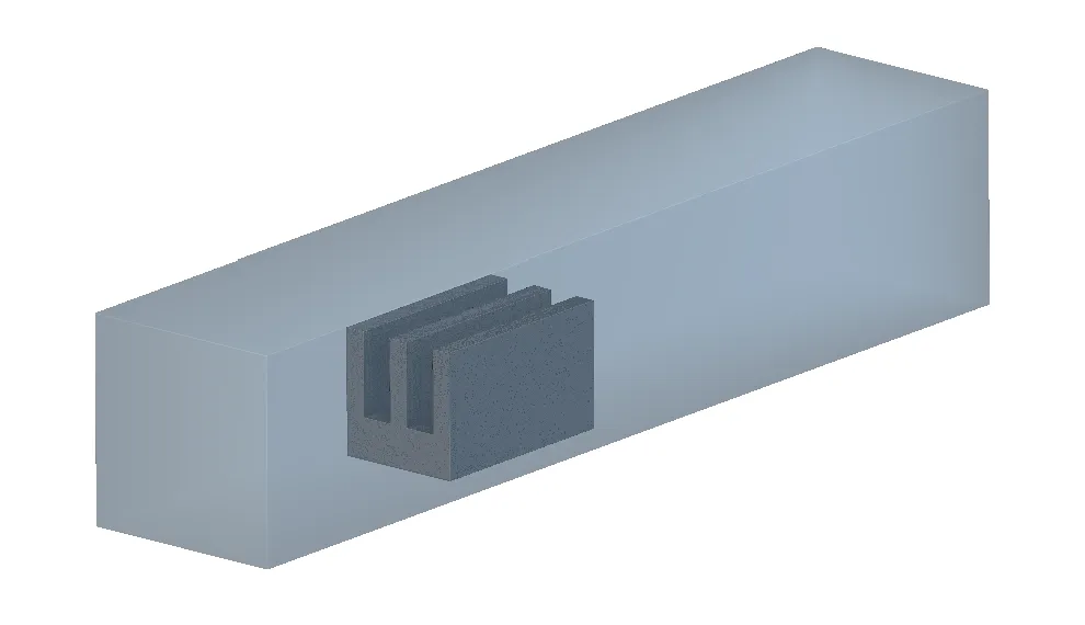
1. Prepare Your Geometry: Before starting, ensure you have implicit bodies defined for both your fluid and solid regions.- Solid Geometry (Heat Sink): The physical parts that conduct heat, such as the heat sink base and fins.
- Fluid Geometry (Air Channel): The negative space or volume surrounding the heat sink where the air flows.
 2. Set Up the Virtual Model: We need to add a Simulation Model block to act as the container for your simulation setup. You will use its “Virtual Model” overload, which is designed for LBM-based simulations that do not require traditional body-fitted meshing.
-
Add the Fluid Domain (Air):
- Add a Fluid Domain block to your Virtual Model list.
- Input your Fluid Domain implicit body as the Body input (the air channel).
- Define the Fluid Attribute using the Air block (or an Isotropic Material: Isotropic Fluid Property (Kinematic Viscosity) and Isotropic Thermal Property (Conductivity and Specific Heat).
-
Add the Solid Domain (Heat Sink):
- Add a Solid Domain block to the same list.
- Input your Solid Geometry (the heat sink body).
- Define the Solid Attribute using an Isotropic Material (e.g., Aluminum) that includes Isotropic Thermal Property values.
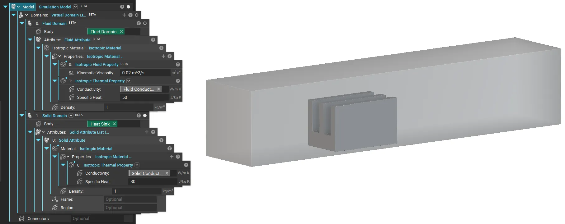 Note: Both materials must have thermal properties defined to enable the CHT solver.
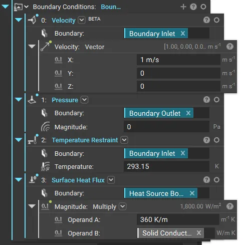
3. Define Boundary Conditions: Input a list of boundary conditions into the Flow Analysis block. For CHT, you need to define both flow and thermal conditions on the relevant CAD faces or boundaries.
Note: Both materials must have thermal properties defined to enable the CHT solver.
3. Define Boundary Conditions: Input a list of boundary conditions into the Flow Analysis block. For CHT, you need to define both flow and thermal conditions on the relevant CAD faces or boundaries.
Note: You need at least one Temperature Restraint to enable CHT.
-
Flow Conditions:
- Inlet: Add a Velocity boundary (e.g., 1 m/s) to the face where air enters the channel.
- Outlet: Add a Pressure boundary (e.g., 0 Pa) to the face where air exits.
-
Thermal Conditions:
- Inlet Temperature: Add a Temperature boundary to the inlet face (e.g., 298 K or 25°C) to define the incoming air temperature.
- Heat Source: Add a Surface Heat Flux boundary to the bottom face of the heat sink base. This simulates the heat load from a chip or electronic component (e.g., 2000 W/m²).
 Note: nTop Fluids automatically handles the heat transfer interface between the fluid and solid domains defined in your Virtual Model. Any wall or boundary not explicitly assigned a thermal boundary condition is treated as having a zero-temperature gradient. This means the solver assumes these surfaces are perfectly insulated, and no heat is conducted across them.
4. Configure the Flow Analysis Block
Note: nTop Fluids automatically handles the heat transfer interface between the fluid and solid domains defined in your Virtual Model. Any wall or boundary not explicitly assigned a thermal boundary condition is treated as having a zero-temperature gradient. This means the solver assumes these surfaces are perfectly insulated, and no heat is conducted across them.
4. Configure the Flow Analysis Block
- Model: Input the Simulation Model containing both the Air and Heat Sink domains.
- Boundary Conditions: Input the list of flow and thermal boundaries created in Step 3.
- Cell Size: Define the resolution of the Cartesian grid (e.g., 5mm).
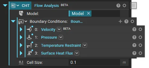 Tip: Use at least 3 cells to resolve the smallest flow features (channels/gaps) and at least 2 cells across solid structures for accurate quantitative results.
5. Run the Simulation: Run the Flow Analysis block.
The solver will automatically couple the fluid and solid equations, calculating how heat dissipates from the source, conducts through the fins.
Tip: Use at least 3 cells to resolve the smallest flow features (channels/gaps) and at least 2 cells across solid structures for accurate quantitative results.
5. Run the Simulation: Run the Flow Analysis block.
The solver will automatically couple the fluid and solid equations, calculating how heat dissipates from the source, conducts through the fins.
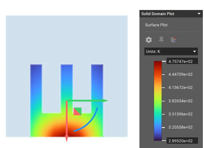
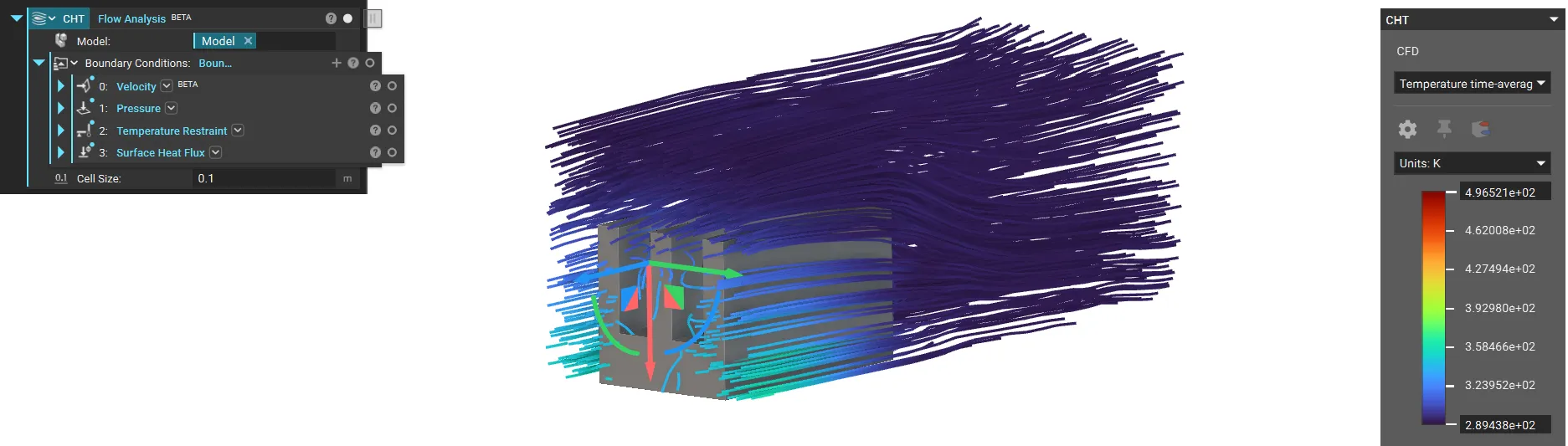 6. Visualize Results: Once the analysis is complete, you can inspect the thermal performance.
- Temperature Fields: Switch the HUD variable to Temperature time-averaged to view the heat distribution on the solid fins and in the surrounding air.
- Display Mode to Streamlines: Visualize the airflow path and color the streamlines by Temperature to see where the air picks up heat.
- Surface Plot: Use the temperature time-averaged field to plot colour onto the implicit body to visualise the values and view them in Section Cut (X) mode.
 And that’s it! You’ve successfully simulated the cooling performance of a heat sink using CHT.
Are you still having issues? Contact the support team, and we’ll be happy to help!
And that’s it! You’ve successfully simulated the cooling performance of a heat sink using CHT.
Are you still having issues? Contact the support team, and we’ll be happy to help!