Question:
How do I use the Remap Constraint for Topology Optimization?
Applies to:
- Remap Constraint
- Topology Optimization
Answer:
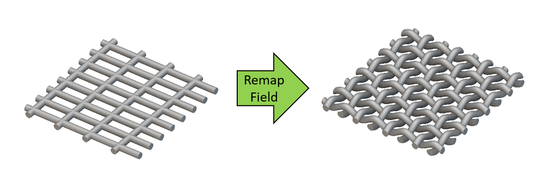
The Remap Constraint block can generate novel geometry with Topology Optimization in nTop. It enforces geometry-based constraints on the design space by leveraging nTop’s unique ability to manipulate scalar and vector fields. The block is named after the Remap Field block that follows a similar technique to perform geometric operations on implicit bodies like shape transformation, mirroring, sectioning, patterning, surface extrudes, and many more applications. Here’s an example of a weave pattern generated from cylindrical wires with the Remap Field block.
 While the Remap Field block can be used to create geometric projections by manipulating scalar fields from implicit bodies, the Remap Constraint block can utilize these projections to constrain the density field of the design volume in an optimization problem. This enables users to impose geometry-based constraints such as extrusion, pattern repetition, and symmetry, combine these constraints or invent a novel constraint that results in an optimized geometry unique to nTop! We recommend that you learn a little about signed distance fields, the inputs of the Remap Field, and the mechanism behind the geometric projections it enables to use the Remap Constraint effectively. This knowledge base video and a learning center course cover these topics in great detail, which will be summarized in the next few paragraphs.
Remap primer
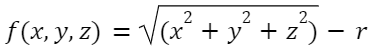
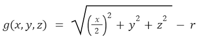
All implicit bodies in nTop are represented as fields called ‘signed distance fields.’ These fields are generated by signed distance functions which are equations that usually represent geometry. For instance, the signed distance function of a sphere of radius ‘r’ at the origin of an orthogonal space is :
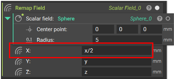
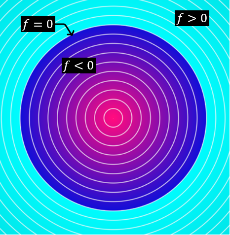 This function evaluates a negative value at every point in space within the sphere and a positive value at every point outside. The sphere’s surface, where the function is 0, is the implicit representation of the sphere. To perform a geometric operation on this sphere, you can manipulate the x, y, z components of this function using the Remap Field block. For instance, to stretch the sphere in the x direction by twice its original length, we can substitute the ‘x’ term in the Remap Field input by ‘x/2’
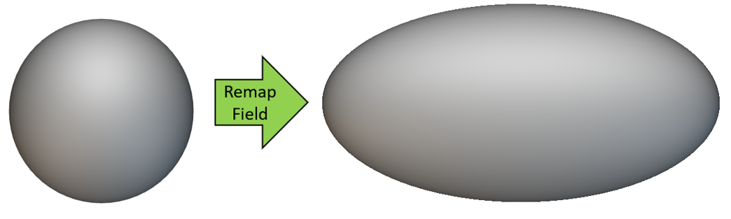 This essentially modifies the field defined by equation f to g to generate an implicit ellipsoid :
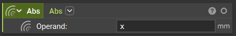
 Besides implicit bodies, visualizing the field generated by each component (x, y, and z) can be used to predict the final state of the implicit body when an operation is performed on a component. In the case of the sphere-to-ellipsoid transformation, the field generated by the x component is stretched (by two times its original value) with the x/2 input in the Remap Field block. Let’s take another example where the x component of the Remap Field input is modified with an Abs() block. The Abs() block outputs the absolute value of a numerical input. Hence the x component will turn into a symmetric signed distance field with positive values on either side of the yz-plane (x=0), as illustrated by the following images.
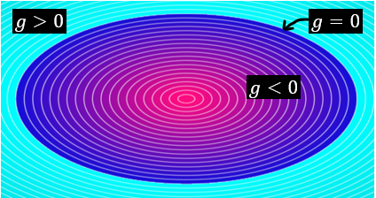
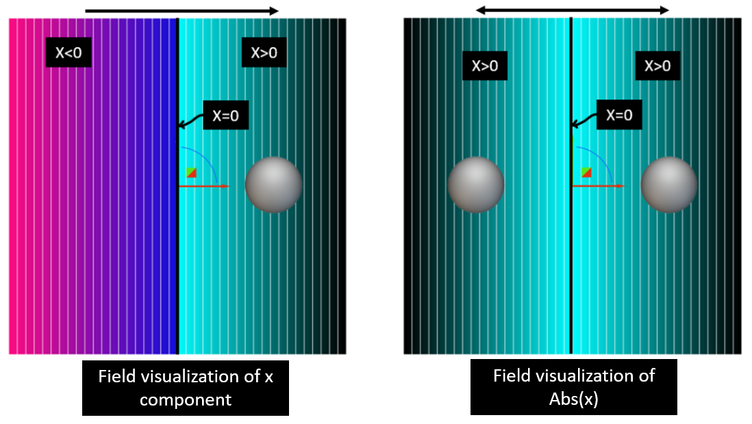 As a result of this field modification, any object created on the right side of the yz-plane will be mirrored to its left side, like the sphere shown in the image above. This concept can be extended to Topology Optimization using the Remap Constraint. We can use the Abs function with any orthogonal components to impose symmetry on the density field generated by the Topology Optimization.
Examples:
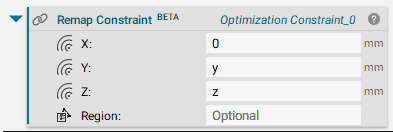
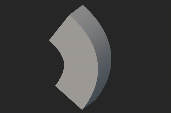
1. Remap Constraint for Symmetry
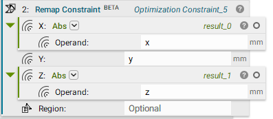
Here is an example of topology optimization with symmetry on the yz-plane (x component) and the xy-plane (z component) enforced by a remap constraint. The equation gives the input to the remap block:
g(x,y,z) = (Abs(x),y,Abs(z))
Tip: Check the orientation of your part before running the Remap Constraint to the global axes.
 Besides the Remap Constraint block, this Topology Optimization setup has the following features that yield the final optimized volume :
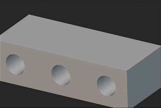
- A minimize Structural Compliance objective for a set of loads at the holes on the sides with the hole at the center completely restrained.
- A Volume Fraction Constraint that keeps the volume of the optimized geometry under 25% of the original design volume.
- A Passive Region Constraint that prevents material removal from the hole at the center.
Example file
Back to top
2. Remap Constraint for Extrusion
Here is an example of a Topology Optimization where the Remap Constraint block maintains a consistent profile along the user-defined direction. This constraint is similar in function to the Extrusion Constraint block for Optimization.
The simplest way to implement this is to set the component input in the desired direction to 0. This will ensure that the field values are constant in the direction normal to the x=0, i.e, the yz-plane. The equation below can represent the input to the Remap Constraint block:
Although these remap inputs work well to produce extrudable geometries in simpler profiles, the general approach to imposing an extrusion constraint with the Remap Constraint block is detailed in Example 4. It possesses several advantages and is qualitatively better than the approach used for this example. More on this in Example 4
Example file
Back to top
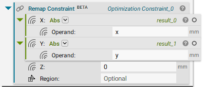
3. Remap Constraint for combining multiple geometric constraints
An essential feature of the Remap Constraint block is the ability to combine multiple geometric constraints in a Topology Optimization. In this example, we have applied an Extrusion Constraint to the z direction and a Symmetry Constraint in the yz- and xz- planes with the Remap Constraint block by combining the inputs discussed in the previous 2 examples. The equation below can represent the input to the remap constraint block:
g(x,y,z) = (Abs(x),Abs(y),0)
4. Remap Constraint for Localized Ribbing
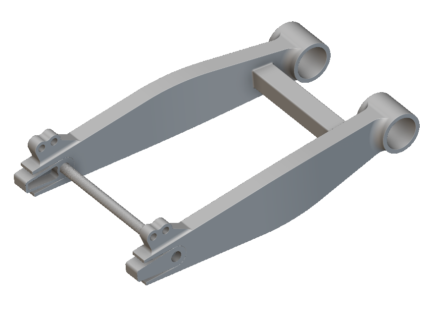
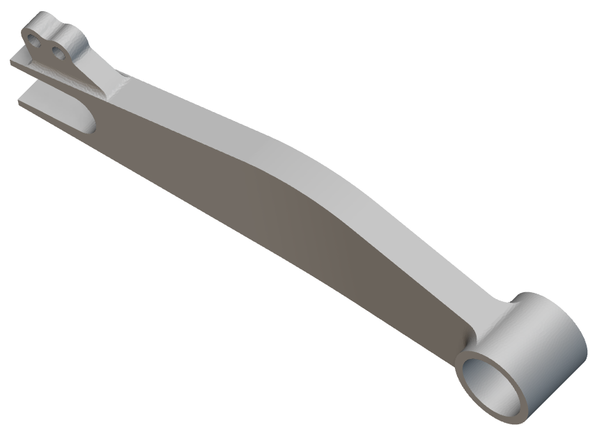
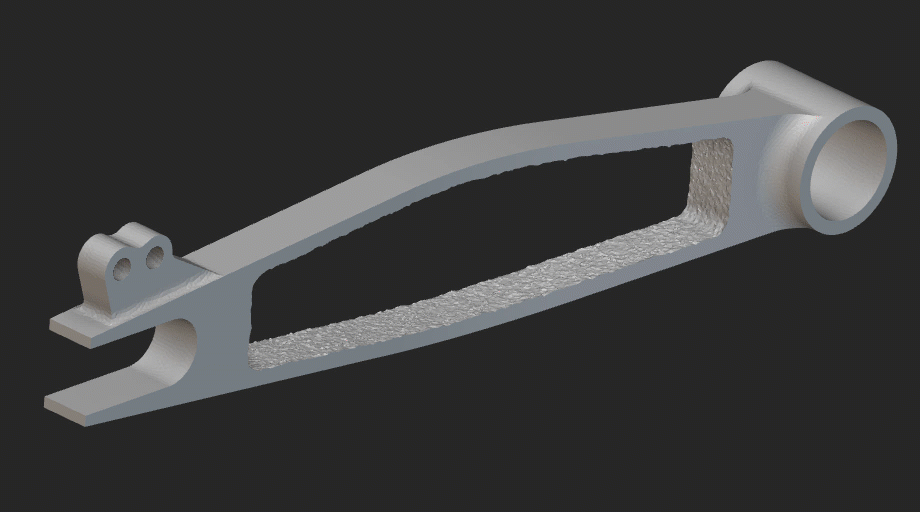
Another essential feature of the Remap Constraint block is to localize a geometry constraint to a user-defined region. In this example, we have optimized a motorcycle swingarm with Topology Optimization to improve the strength-to-weight performance. The Remap Constraint block was utilized to apply a localized extrusion constraint to generate ribs. This would enable the swingarm component to be manufacturable through non-additive methods such as casting.
 Unlike the previous examples, the Extrusion Constraint has been implemented using a generalized form that the equation can describe:
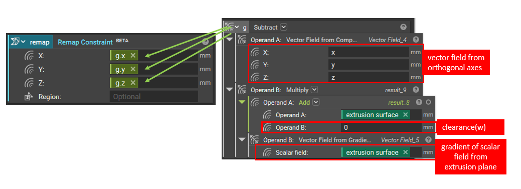
This generalized form allows the Remap Constraint block to determine the extrusion direction based on optimized surface normals of the design volume. We can decompose the equation into the following parts to understand how this is implemented :
Unlike the previous examples, the Extrusion Constraint has been implemented using a generalized form that the equation can describe:
This generalized form allows the Remap Constraint block to determine the extrusion direction based on optimized surface normals of the design volume. We can decompose the equation into the following parts to understand how this is implemented :
- x represents the position vector of all points in the orthogonal space (x,y,z).
- s(x) represents the surface, the signed distance field to the reference surface from which we extrude. This is usually an implicit surface extracted from the geometry being optimized. A value of w is added to ensure that the remapped field is within the user-defined design space being optimized.
- ∇s(x) (the surface gradient, s) extracts the vector field representing the extrusion profile’s surface normal. Multiplying this by s(x) (the scalar field of the implicit surface) produces a vector field that projects any point, x, back to this surface.
Ultimately, we use the remap block to extract a field with a constant value and direction determined by the extrusion surface. This field can also be generated by a proxy surface that lies within the cross-sectional area of the optimized design volume. Here’s a field viewer visualization of remapping a noise field (left) using the equation with a cylinder as the surface.
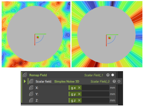 The noise field (left) is remapped to the field (right) with a constant value in the surface in the normal direction of the cylinder. There are several benefits to using this generalized approach as opposed to the simplified approach described in previous examples (Examples 2 & 3), a few of them being :
- The ability to apply multiple extrusion directions in the same optimization.
- The ability to utilize non-planar extrusion surfaces in the optimization problem.
In addition to the Remap constraint, the optimization setup in this example has the following inputs :
- An objective is to minimize the compliance of the model for a set of boundary conditions
- A volume fraction constraint to keep the volume of the optimized volume under 50% of the initial volume.
The following animation illustrates the final shape of the design with extrudable features that maximize the stiffness of the model:
 Example file
Back to top
Example file
Back to top
Keywords:
field topology question optimization constraint remap remapping