Objective:
Learn how to run a field optimization.
Procedure:
What is Field Optimization?
Field optimization is a numerical design operation that optimizes design parameter values within the bounds of a design space (based on a set of objectives and constraints). Field optimization allows the user to run an optimization algorithm on specific parameters, such as lattice or shell thickness, to achieve the best geometry for the desired objective (while considering complex and multivariate design constraints).
Before starting with field optimization, we have two requirements: FE Volume Mesh and Boundary Conditions (BCs) to apply the Constraints. Follow the instructions in the links below to prepare your model for field optimization.
FE Mesh
- How to create an FE Volume Mesh
Boundary Conditions (BCs)
- How to choose boundaries of an FE Mesh - FE Boundary by Body
- How to Use Boundary Conditions
- How to use a CAD Face in a boundary condition
1. Creating a Parametric FE Model
Follow this link to learn about FE Models and how to create them. The Parametric FE Model would need one of the Parametric Domains as an input.
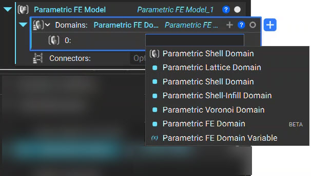 What Parametric Domains are available? 4 Parametric Domains could be used as an input to the Parametric FE Model. You would have to choose a domain based on what you wish to optimize and achieve. You can learn more about each domain and how it is parameterized by clicking the Learn More link on the block.
| Parametric Domain | Visual Representation | Design Parameters | Field Optimizable Design Parameters |
| Parametric Lattice Domain | 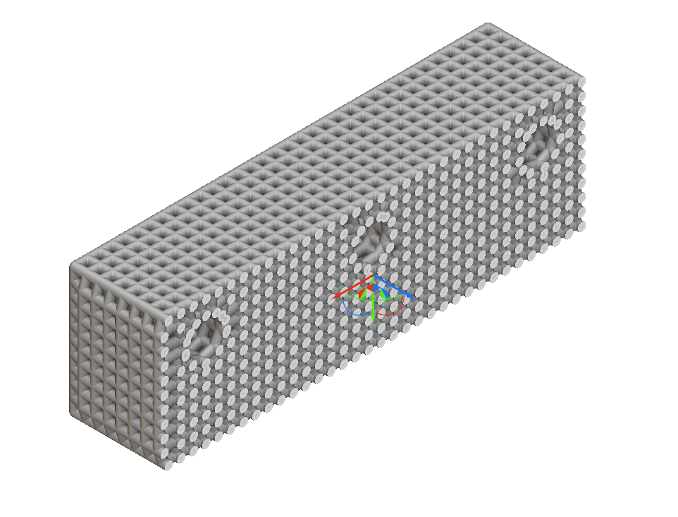 | Unit Cell, Boundary Behaviour, Cell Size | |
| Parametric Shell Domain | 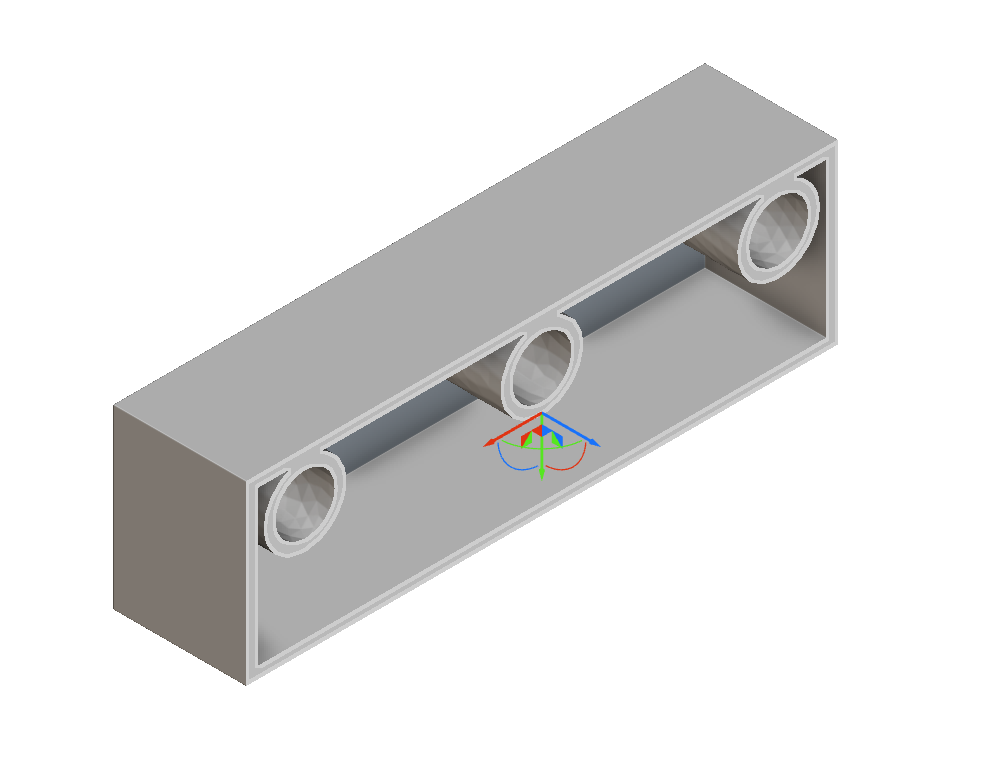 | | - Min and Max Shell Thickness
|
| Parametric Shell-Infill Domain | 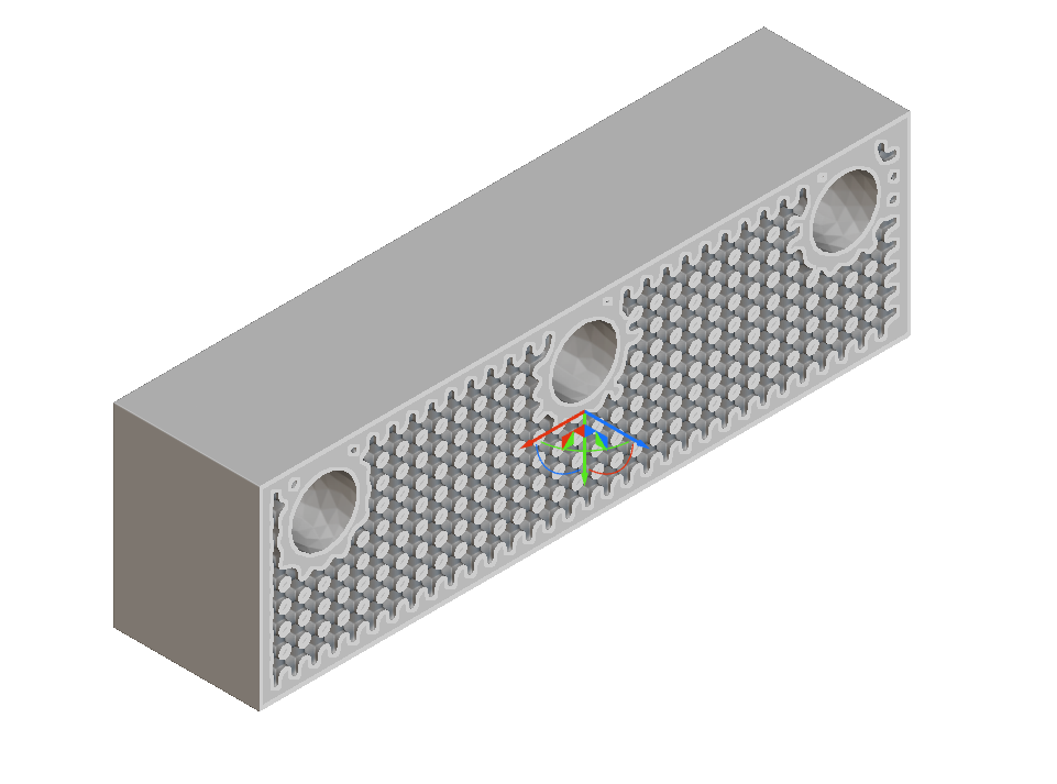 | Unit Cell, Cell Size | - Min and Max Infill Thickness
- Min and Max Shell Thickness
|
| Parametric Voronoi Domain | 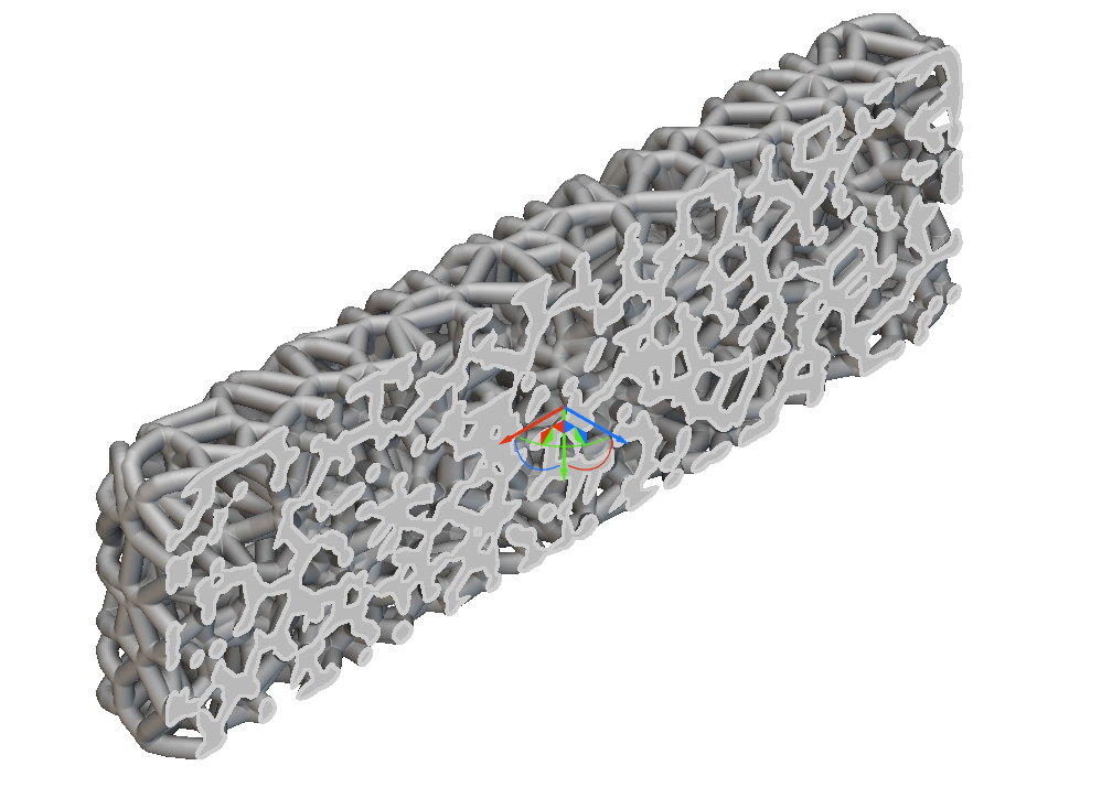 | | - Min and Max Cell Size
- Min and Max Thickness
|
Tip: If you wish to optimize only the Thickness instead of the Cell size in a Parametric Voronoi Domain, use a constant Cell size value for Min and Max.
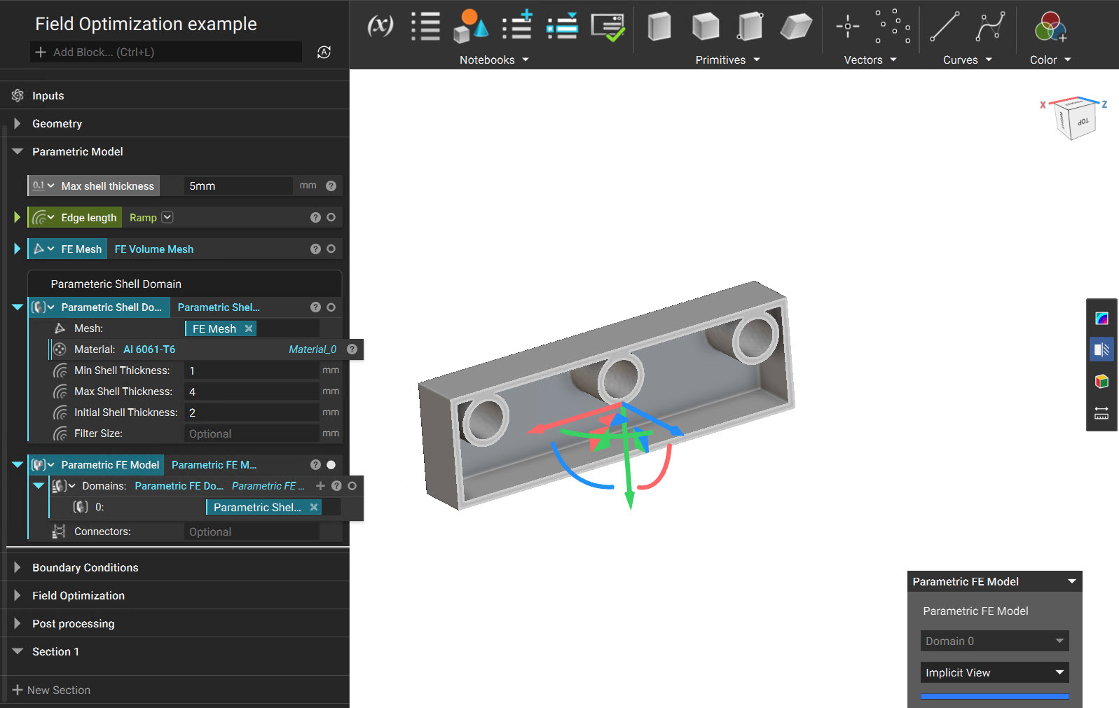
- Implicit view - allows you to view the resulting geometry by changing the Initial values in the input of the Parametric Domain block.
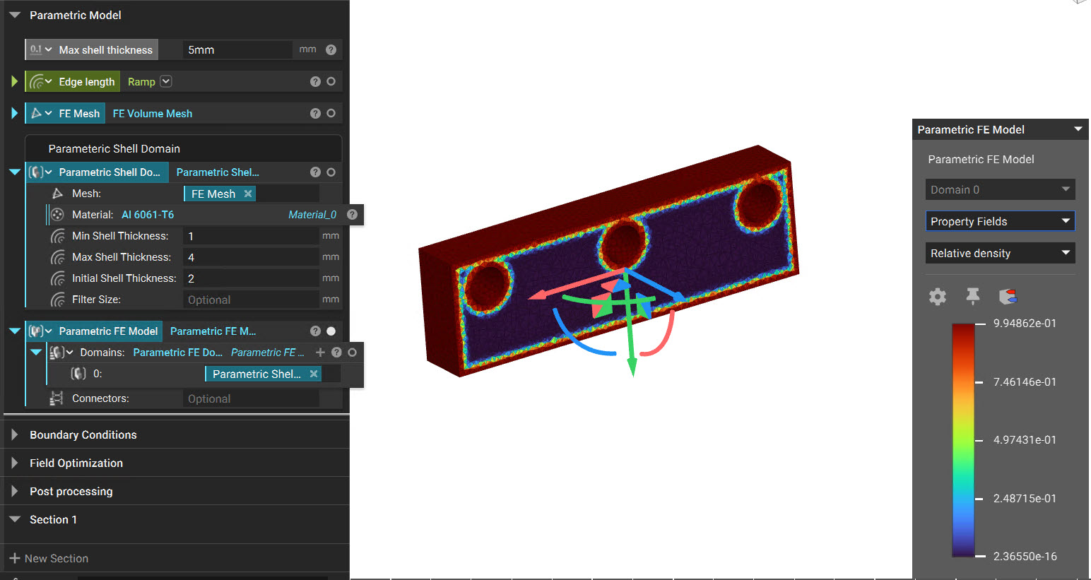
- Property Fields - allows a user to view the homogenized mechanical properties of the structure across the design space before performing field optimization. The properties that can be accessed from the HUD are Relative density, Density, Young’s Modulus, Poisson’s Ratio, and Shear Modulus.
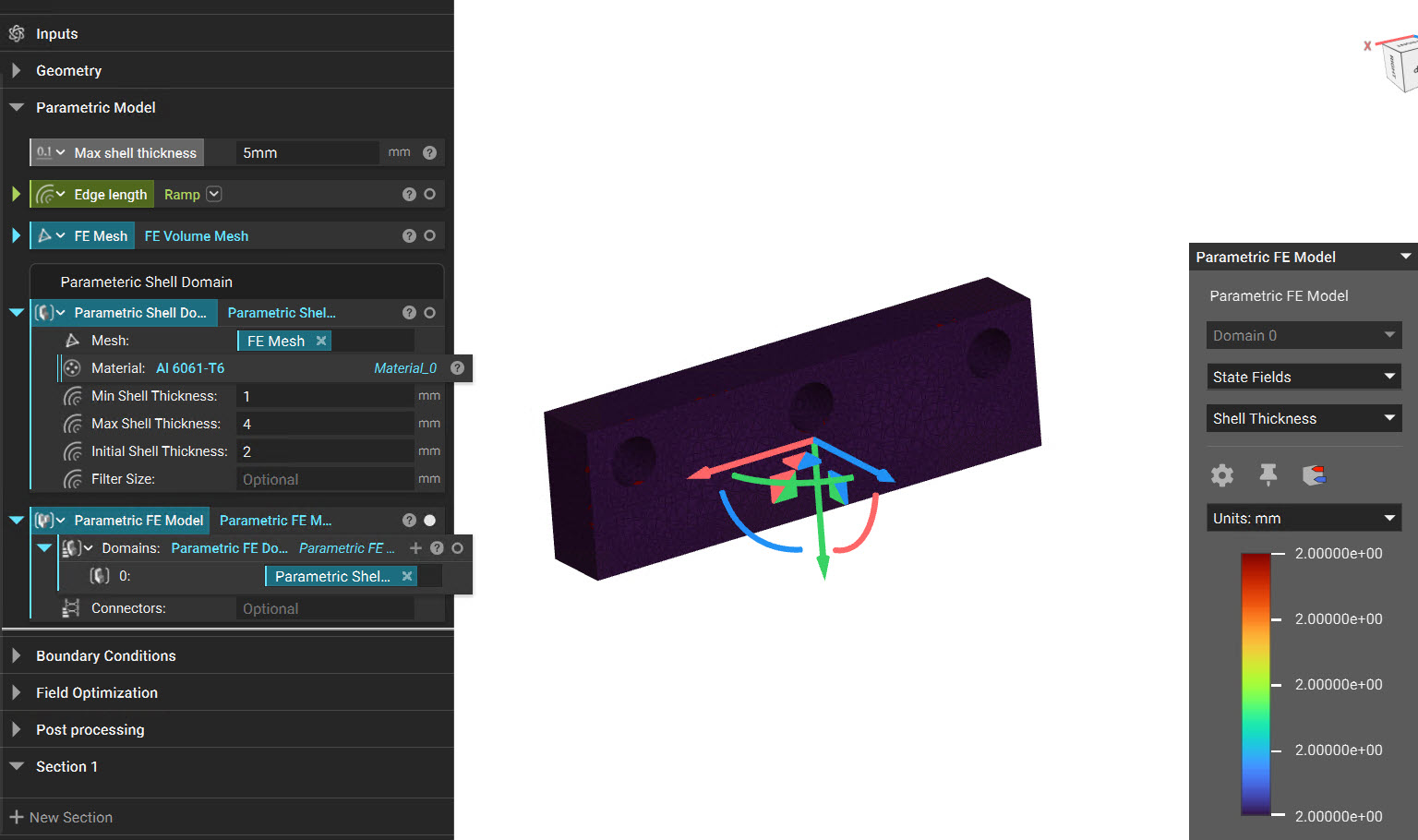
- State Fields - allows a user to view values of the design parameters across the design space before performing the field optimization. For example, in this case, the controllable design parameter is thickness which would be the same as our Initial input value.
2. Define the Objective
The Optimization objective is what property, or ‘Design Response,’ we hope to minimize or maximize within our part. nTop supports several design responses, including Structural Compliance, Volume Fraction, Displacement, and Stress.
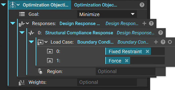
Use the Optimization Objective block to specify the design response(s). In this example, the objective is to minimize structural compliance.
- Add a Structural Compliance Response block.
- Insert the Displacement Restraint and the Force block.
- Add an Optimization Objective block
- Set the goal to Minimize
- Insert the Structural Compliance Response into the Design Response List
3. Define the Constraint
Field optimization can also take constraints as input. Without Constraints, the optimization will probably result in parameter values at their maximum/minimum bounds. Constraints can include upper or lower limits on other Design Responses and others.
The most commonly used constraint applies a minimum or maximum bound to a design response, such as compliance, volume fraction, displacement, or stress.
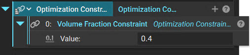
This field optimization example is constrained such that the volume fraction of the final part is less than 0.4. In other words, the resulting optimized part will have a targeted volume of 40% of the whole design space. Notice that the volume fraction cutoff in the Design Response Constraint block is a variable for easy adjustment.
- Add an Optimization Constraint List block
- Insert a Design Response Constraint block
- Insert a Volume Fraction Response block into the Response input
- Set the value to .4
- Optional: Right-click on the Value input to create a variable to change the Volume Fraction quickly.
4. Run the Field Optimization
- Add a Field Optimization block,
- Insert the Parametric FE Model
- Insert the Objective
- Insert the Constraints
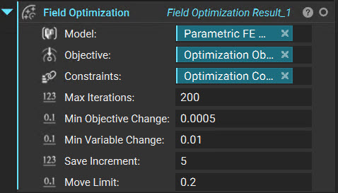 You can leave the rest of the inputs as default for this example. You can find more information on these settings in the block’s information panel and in this article. After completion of field optimization processing, a window appears in the Viewport with several options for visualizing the results.
- Implicit view - allows you to view the resulting geometry. Under the “render, as needed” drop-down, each iteration will render when you move the slider bar. Use the “render all” option in the drop-down to render more than 1 iteration at a time to view the progression of the field optimization results easily.
- Property Fields - allows you to view the mechanical properties of the resulting structure across the design space. You can display the results across the original mesh and render them in real time for any saved iteration.
- State Fields - allows you to view values of the design parameters across the design space. You can display the results across the original mesh and render them in real time for any saved iteration.
5. Field Optimization Post-Processing
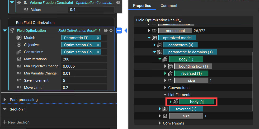
To get the resultant Implicit Body, you must grab the Implicit chip from the Properties panel (optimized model > parametric fe domains > Properties > body).
- Add a Boolean Union block
- Input the Smoothened Body and the Interface Bodies
- Set the Blend radius to 2 mm (to keep the transitions between bodies congruent)
Lastly, perform a Boolean Intersect operation with your part and the original CAD body to ensure that you preserve the interfaces of the original design space.
And that’s it! You’ve successfully performed a field optimization.
Are you still having issues? Contact the support team, and we’ll be happy to help!
Download the Example file:
Keywords:
FE voronoi field variable how infill optimization setup to run Parametric shelling Components