
- Define the wing’s leading and trailing edges to set up the planform.
- Assign an airfoil using a profile.
- Parameterize the edges to stretch and position the airfoil profile along the wingspan.
- Mirror the wing setup to generate symmetric wings.
- Generate solid, planar wings using a bounding box to trim the wing to the planform shape.
- Twist the wings from root to tip.
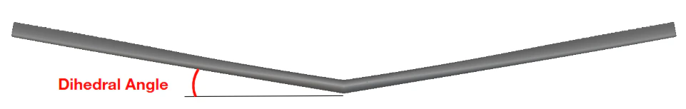
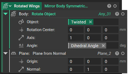
- Rotate the wings to account for the dihedral angle.
1. Edges
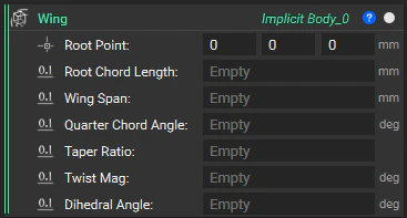
Define the wing’s leading and trailing edges to set up the planform. Let’s begin by defining the general shape of our wings by creating two curves: one for the leading edge and one for the trailing edge. We will keep our modeling operations as simple as possible. Since wings are symmetric, we can begin by modeling the edges of only one wing. We’ll mirror this initial geometry later on. The diagram below shows the curves we want to generate to define the highlighted in blue. This is a good opportunity to make a custom block, as many of the parameters that go into this can be used in other aircraft workflows. We will set up the block using the five parameters laid out in the diagram.
- Root Point: The frontmost point where the wing attaches to the fuselage.
- Root Chord Length: Wing length from front to back at the root.
- Wing Span: Full span of both wings.
- Quarter Chord Angle: Sweep angle measured at 25% chord line; positive values sweep back, negative sweep forward.
- Taper Ratio: How much the wing narrows from root to tip.
Transcript
Transcript
Let’s walk through making this custom block to generate the leading and trailing edges of this single panel wing. Note that the output of this block is the leading edge and the trailing edge of only one of the wings, and later on we’ll mirror the wing across the fuselage.We’ll start with the inputs laid out in this diagram. Run a couple of calculations to help us parameterize our model and then generate our quarter chord, then building our leading and trailing edges around that. Since we’re beginning by modeling only half of our platform, we’ll start by dividing our full wingspan by two, generating a half wingspan variable. And we’ve input our root cord length, but we’ll need a tip cord length by multiplying that root cord by the taper ratio. Now, we have all the inputs and calculations that we need to generate our quarter cord and our leading and trailing edges.To make a quarter cord or the cord that’s 1/4 away from the leading to the trailing edge, we’ll create two points: QC point and QC point 2. We want to orient this platform on the XY plane so that the fuselage runs along the X-axis. So what we can do to create the first quarter cord point is translate our root point some distance along the X-axis. In this case, that would be 25% of our root chord length. So, all we have to do is translate our object by this vector where we multiply the root cord length by 0.25. So, now if we look at our root point, which is at 0 0, we see our translated point some distance along our x-axis.To make our second quarter cord point, we’ll want to translate that initial QC point, half the wingspan in the Y direction, and some distance further in the X direction. To determine that X, we’ll multiply the half wingspan by the tangent of the quarter cord angle. We’ll keep our Z component at 0 mm to ensure our result is all co-planar. We’ll check the visibility of that chord. And now if we feed our QC1 and QC2 into a Line block, we’ve generated our quarter cord.Now moving forward to the leading edge, we’ll do something similar. We already have our root point, which will feed into the first point of the line that creates our leading edge. To generate the second point, all we’ll do is translate that second quarter cord point a quarter of our tip cord length in the X direction. That generates this point, which we can feed into our Line block to generate that leading edge.For the trailing edge, we’ll again do something similar. First translating our root point by our root cord length to make our initial point and then translating our QC point 2 by 3/4 our tip cord length that’ll generate this second point which we can feed into our Line block to generate our trailing edge.Now viewing this from the top, we can imagine our fuselage here on the left side of these lines, and we can feed our leading and trailing edges into a Curve List. Set those as our output. And now we finished creating this custom block. And because we set this up parametrically, we can now go into our inputs and change any of these around. Maybe adjusting our wingspan or our quarter cord angle to test out different variations of our leading and trailing edges.
2. Profile
Assign an airfoil using a profile.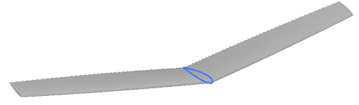
- Freehand approach: Manually define control points and splines for complete creative control
- Parametric approach: Use mathematical equations and predefined airfoil generators
Transcript
Transcript
Now, let’s walk through two different scenarios of setting up your airfoil profiles. In the first option, we’ll use a freehand approach where we create one spline, mirror it, and then generate a profile from it. In the other, we’ll explore a parameterized custom block that allows you to enter a four-digit NACA code and outputs an airfoil profile on its own.Something to keep in mind here is that we’re modeling with implicit bodies and scalar fields. So the result of this section needs to be a profile with its own sign distance field. That means that later on when we want to remap or apply other field operations to it, we won’t run into any issues.Let’s start with our more freehand approach where we create a spline by control points and then mirror that spline to our notebook. We can add a Spline by Control Points block. Then we can add any number of points that we want. I’ll add a Point List and we’ll include five input points.Let’s make our leading edge fall right where our root point was in the beginning. We can take that root point and drop it in as control point number one. Then maybe for our next control point, we can drag it up in the Z direction a bit. Next, maybe we’ll adjust the X and the Z. We’ll do the same for the next point. And then maybe our final point or our trailing edge can take into account our root cord length. So, we can right-click and maybe convert this to a Point block and use our root chord length as our X. That’ll place this final point here at the end. Viewing this from the side, we’ll have a point list that looks something like this and a spline that turns out like this.Now, say we want to take that spline and mirror it. We can build that out together or we can just use the custom block that we’ve provided. I’ll pull in the Mirror Spline custom block and add it to my notebook. And if we right click and open this up, we can see what’s going on in here. So, we have a spline that we input and the plane that we mirror it across. And what this block is going to do is take those control points out of your spline and translate each of them by some distance. To define that distance, we use the Evaluate Field block where we take the field of the plane and evaluate that field of each of those points.Since the field is just an SDF of the plane itself, each of those evaluated values just represents the distance of the points from that plane. So then when we translate those points, we can just take the unit vector of that plane’s normal and drag each point in the negative direction. Here we use a multiplier of two. The first instance pulling the points back to the plane surface and the second instance pulling them that same distance opposite the plane. Finally, we take those translated points and feed them into a new Spline by Control Points block to generate our mirrored spline. Keep in mind here that will also retain the degree of our initial spline.So if we come back here into our original notebook, we can make that Spline by Control Points into a variable called top spline, drag it into our mirror block and generate some plane. So viewing this from the side, we see that we have our initial top spline that gets mirrored.I’ll take this mirrored spline, right click to make it into a bottom spline variable. And then if we view the field of each of those splines, we see that we have these unbounded curve fields on the bottom and the top. So our last step here to create one cohesive profile with assigned distance field is to add the Profile from Curves block. Drag our splines into our curve list and view our resulting field. Now we have this fully enclosed profile with that negative on the inside, positive on the outside, and this infinite field in the Y direction. I’ll right click and make this into a variable called airfoil profile.So you can go about making your own airfoils, creating your own splines, and making your own profiles, or feel free to explore or create your own parameterized custom blocks to generate profiles on your own. One example you can download in the example files is this NACA four-digit airfoil creator that generates these NACA profiles depending on a four-digit code that you input. You can play around with this and see the types of airfoils you can create. I’ll right-click and make this into a variable called NACA profile. And now we’re familiar with these two different approaches.
Tip:
You can explore building and using pre-defined airfoil profiles like we see in the NACA airfoil profile generator below. Use 4-digit NACA codes to generate the profile, and plug into your own wing generators in the future!
You can explore building and using pre-defined airfoil profiles like we see in the NACA airfoil profile generator below. Use 4-digit NACA codes to generate the profile, and plug into your own wing generators in the future!
3. Parameterization
Parameterize the edges to stretch and position the airfoil profile along the wingspan. Now, we have defined our leading and trailing edges and the airfoil profile that will follow them. At the wing’s root, the airfoil profile perfectly represents the surface. However, the profile will need to vary from root to tip to accommodate for the wing’s taper.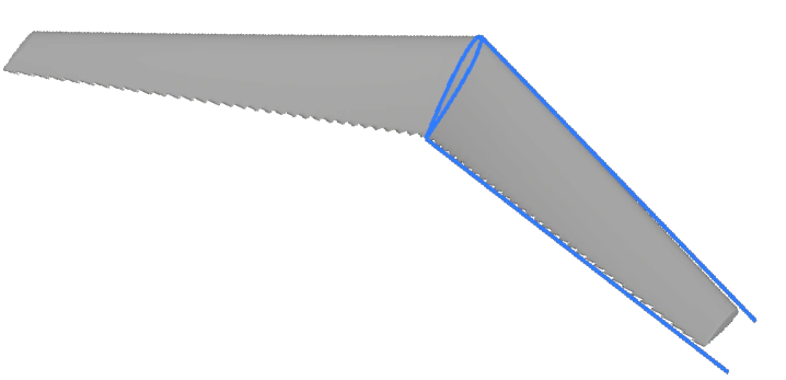

Transcript
Transcript
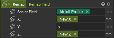
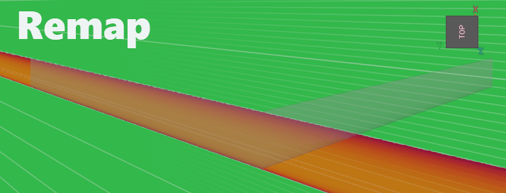
By this point, we’ve defined our leading and trailing edges, and we have the airfoil profile that we want to extrude along these edges. If we look at the field of this airfoil profile, change our color map to an implicit, and add our isolines in, we see that we’ve got this constant field that follows the Y-axis. Now we want to take this field and morph it so that it falls between the leading and the trailing edges.To do this, we’ll have to take that profile and remap its X and Z components to scale that profile as it moves along the Y direction. The results of our Remap Field block should look something like this. Note that our new isolines would remap so that they’re conformal between the leading and trailing edges. And we have a new X and Z component while our Y is going to stay the same. So in this parameterization section, we’ll see our new X, our new Z, and the same Y that we had in our original airfoil profile. Let’s start with the new X. Here we’ll use the custom block provided called Single Panel Wing Parameterization. Our inputs here will be the leading and trailing edges and our root chord length.Right-clicking and opening this custom block, we can see the underlying operations. We start with two fields, one for our leading edge and one for our trailing edge. And these are just going to be sign distance fields radiating from either of those two curves. We then use the Distance To Curve From Axis block to measure each curve’s distance from the Y-axis along the X direction. This will output two separate scalar fields, one for the distance to the leading edge and one for the distance to the trailing edge. We then feed these into scalar fields A and B where in A we would subtract X from the distance to the leading edge and multiply that by -1. And in B we would just subtract X from the distance to the trailing edge.Let’s look at an example of what this might look like. I’ll scroll to the top just to test this out, double click and add my single panel wing edges just to create a test case. And from my list elements, I’ll want to pull in my leading edge and my trailing edge. I’ll pull these into my notebook and pull them in to test.Now, if I look at my distance to leading edge, I’ll see a field that looks like this. Starting at zero and moving to 800 or half of my wingspan, my distance to trailing edge field will look like this. My A field will look like this and my B will look like this. Now I take that A and B and feed them into this Two Body Field block that essentially finds the midsurface between those two A and B input fields. To look further into that Two Body Field block, you can always right-click and open your custom block.Now from that field, I see that I’m at zero at my center, -1 at that trailing edge and positive one at the leading edge. To pull that zero to one of my edges, then all I have to do is subtract one from the field we’re viewing. And now I see that my zero falls along this leading edge. Now my field ranges from 0 down to -2. And if I take my root chord length and divide it by -2, then multiply by the field we’re viewing, I’ll see this result. My field now spans from zero at my leading edge to about 1,200 at my trailing edge. This is going to be my new parameterized X field. So going back into my notebook, I can take that new X and drop it into our remapped field.For my new Z, I can expand this block and I can again use this Distance To Curve From Axis block. We’ll now measure our distance in the X direction to the Y axis from our trailing edge and from our leading edge. We’ll subtract the leading from the trailing then divide by our root chord length.Now we see the field equal to one at our original profile and 0.5 at the tip of our wing. Note that this is going to match our taper ratio of 0.5. We then take the reciprocal by dividing that by 1. And now we go from 1 to two at our tip. We can multiply that by Z. And if we take that new Z and drop it into our remap block, that’ll mean that the Z height scales in this case by 0.5.Now, viewing the results of our remapped field, I can use the Field Viewer and see how my X and my Z have scaled along this Y direction.
4. Symmetric Mirror
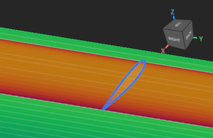
Mirror the wing setup to generate symmetric wings. Remember, the Remap field only applies to one half of our full wing setup. For the rest of our modeling operations, we want to use both halves of the wing. To do this, we need to mirror our Remap field. A standard Mirror Body block won’t work because it reflects the entire field and would return only the opposite wing, leaving us with the same issue as we see to the right: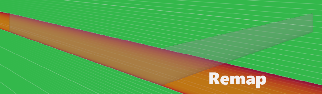
Transcript
Transcript
By now, in our platform setup, we’ve set up our leading and trailing edges, created our airfoil profile, and then remapped our initial implicit field to a newly parameterized field in the X and Z directions. Up to this point, we’ve only been working with half of our platform, or one of our wings, for our aircraft. Now, we’ve come to the point in our setup where we want to mirror that wing and work with both wings.From now on, if I were to take this remapped field and drop it into a Mirror block, I could assign some plane for it to mirror across, and the result would represent our opposite wing, and we would be faced with the same problem. What we’ll actually need to do is set one side of that remapped field to its actual values and the side opposite the plane to zero. From there, we can mirror the field, and we’ll get an accurate representation of what our platform’s field should look like.You can build this on your own, or we can use this Mirror Body Symmetrically custom block. We’ll open our custom block to see how it looks. We have our body input, or the implicit body or scalar field that we want to mirror, and the plane about which we want to mirror it. Let’s test this custom block out with a simple example. I’ll add a box to our notebook and drag our plane and our body into our notebook to test it out.I’ll drag our box to one side of our plane and make it our body input for now. Viewing its field and adjusting that size, I see that we’ve got this one implicit field, and we want to mirror it across our plane. We’ll have to do a couple of setup steps first. We’ll start by representing the coordinate system, or the field that we want to mirror, using this Vector Field From Components block and simply inputting X, Y, and Z.Now, we’ll want to calculate the signed distance from any point to our plane, but clamp our negative values to zero. What we can do is subtract our plane origin from this P field, then find the dot product between that difference and the negative normal of our plane. That outputs a flipped version of our plane that we can then feed into a Max block. So now we’ve set the underside of our plane to have positive values and the top side of our plane to be clamped to zero.Next, we can multiply this field by -2 to adjust its scale, multiply by the negative normal of our mirror plane, and add that initial P vector field. Finally, we can take that body and remap it to the X, Y, and Z components of our P field. And now we have our mirrored result: our original field on the top side of our plane, and the symmetrically mirrored field on the bottom side.Jumping back into our original notebook, we see that we can take our original remap, feed it into that Mirror Body Symmetrically block, include our mirror plane, and now we have that symmetrical planform.
5. Planar
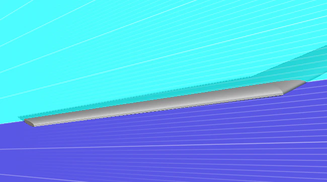
Generate solid, planar wings using a bounding box to trim the wing to the planform shape. Up to this point, we have only been working with unbounded scalar fields and have not yet created enclosed, implicit geometry. Let’s generate an enclosed profile, then use its properties to make a bounding box to intersect with our scalar field from above. Feel free to take a look at the video and custom block below.
Transcript
Transcript
Now we have the underlying scalar field for our wings, but our field is unbounded. So we don’t actually have an implicit body yet. Let’s take this field and some of the data that we already have to generate an implicit body representing our wings.We’ll start by generating our wing plan form as a profile. This profile will be made up of six curves: two each for the leading and trailing edges and one each for the wing tips. We’ll start with a line for our first wing tip, which just extends from the end point of our leading edge to the end point of our trailing edge. We can then mirror that line using this simple Mirror Line block that just mirrors our start and end points across a plane and generates a new line from the result.Then we’ll add in our leading edge and our trailing edge and then rotate each of those using the Rotate Object blocks. We’ll rotate those 180° around our x-axis or our fuselage. Our result will be a platform that looks like this. And we can use that profile’s dimensions to generate some implicit body that we can then intersect with our scalar field that we created in our previous section, resulting in a solid body.We’ll take the minimum and the maximum x components of our points from that profile. Assign our Y components as the positive and negative halves of our wingspan and use the maximum and minimum Z components of our air foil profile to create this box from corners. From there, we can just intersect our box with that mirrored wings field that we created before.Viewing our box in transparent mode, we now see where the intersection will happen. We’ll use our Boolean Intersect block to generate those wings.And then we’ll translate that object by our root point vector. Since we’ve set our root point to the global origin, this won’t actually move our intersect, but it’s good practice for parameterization and generalizing our custom blocks.
6. Twist
Twist the wings from root to tip. To drive lift distribution, we want to twist the wing. The result should look something like this, where the wing twists about the mid-curve from root to tip. Use the custom blocks and watch the videos below to identify the mid-curve and twist the wing.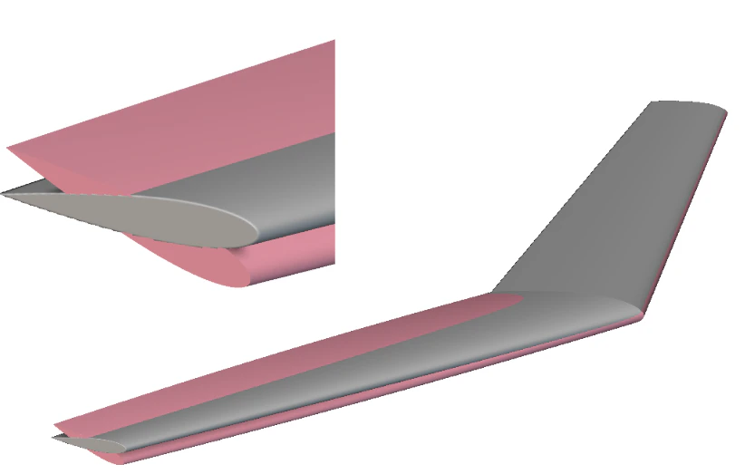
7. Rotate
Rotate the wings to account for the dihedral angle.