Analysis at the Mesoscopic Scale
We can approach fluid dynamics at three distinct scales: microscopic, mesoscopic, and macroscopic.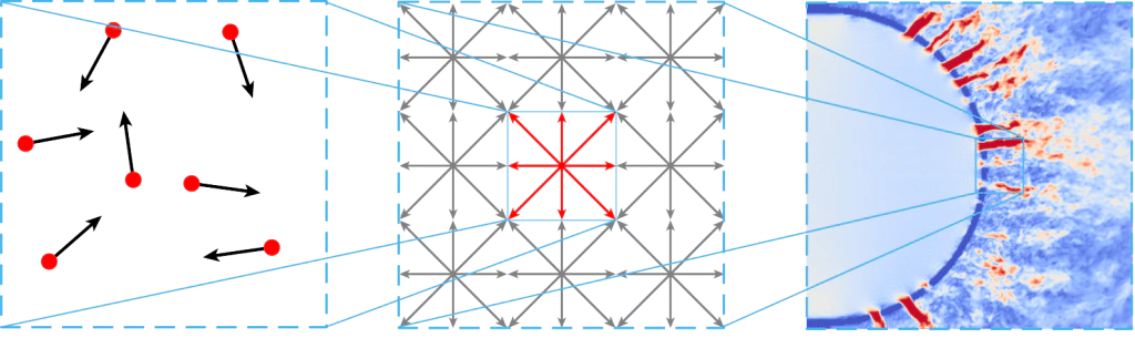
- Microscopic
- Mesoscopic
- Macroscopic
Approaching fluid dynamics at the microscopic view uses molecular dynamics, tracking the movement and interactions of individual atoms or molecules, governed by Newton’s laws of motion.This approach is computationally intensive, limiting its application to very small spatial and temporal scales or specialized applications where molecular-level interactions are crucial.
Discretization for LBM
Rather than relying on complex and computationally expensive meshing algorithms, LBM models efficiently subdivide a fluid domain into a Cartesian grid composed of equally sized cells. Each cell represents a discrete location where the particle distribution functions are tracked.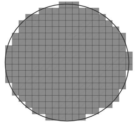

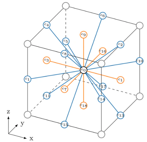
- f: discrete particle distribution function
- c: discrete velocity
- x: position
- t: time
- Ω: collision operator
- m = number of discrete velocities
- n = number of dimensions (2D or 3D)
Collision and Streaming
There are two major steps in the LBM algorithm, collision and streaming, that represent fluid particle behavior at each of these discrete locations.
GPU Implementation & Parallel Computing
nTop’s implementation of LBM on GPUs unlocks dramatically faster simulation times; often 10-100x faster than CPU implementations. The chart to the right shows performance on two NVIDIA GPUs. 1000 Million Lattice Updates per second (MLUPs) means that you can compute 1000 Iterations on 1 million cells in one second.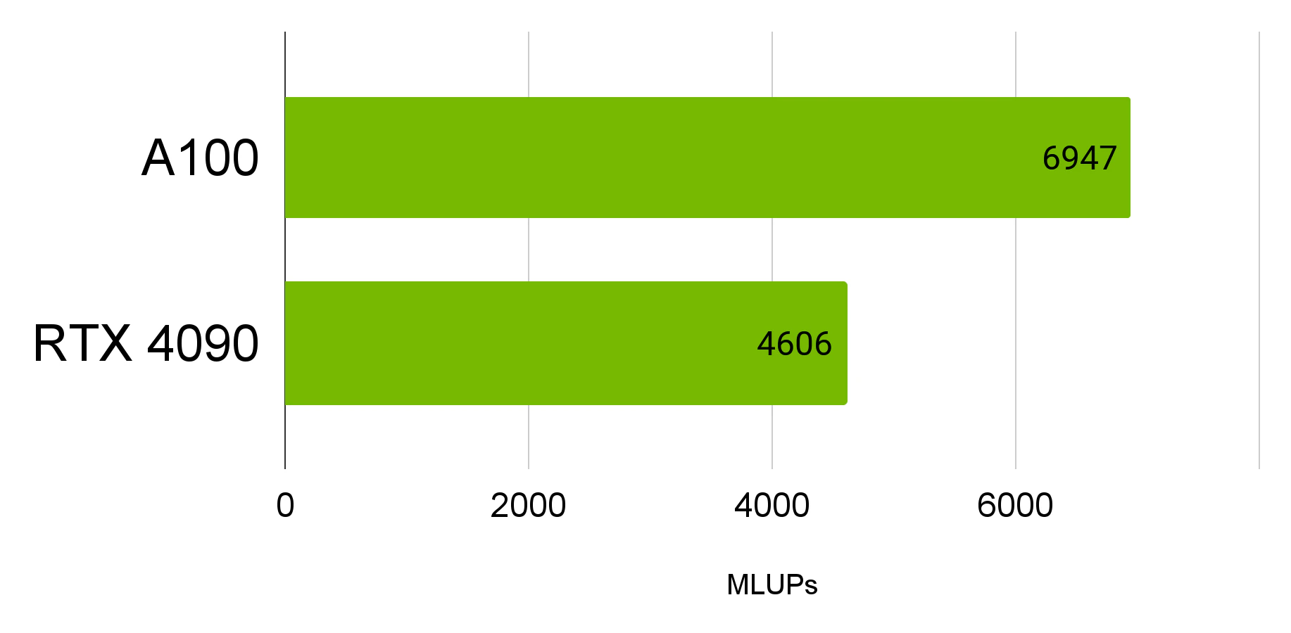
This allows users to handle larger, more complex simulation domains without prohibitive runtime, and to achieve real-time or near-real-time results for certain problem sizes, enabling interactive exploration.