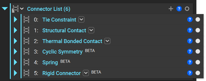
You will need connectors if you are working with multiple domains in your Simulation Model. We have six types of connectors: Tie Constraint, Structural Contact, Thermal Bonded Contact, Cyclic Symmetry, Spring, and Rigid Connector.
Tie Constraint
A Tie Constraint is a rigid connection that ties two nodes together. Tie constraints make the displacement of the selected nodes equivalent, effectively removing one degree of freedom from the system.
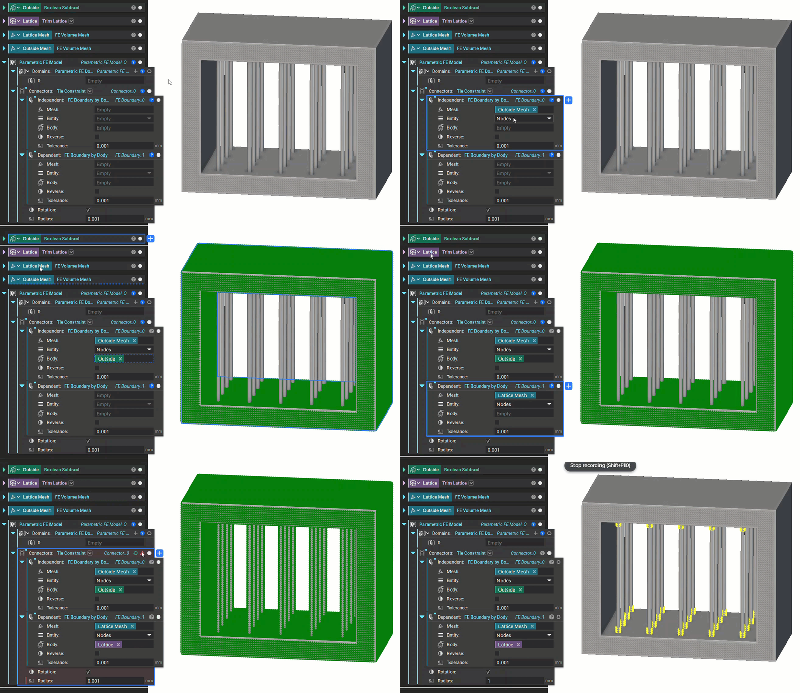
Choose the Independent nodes and the Dependent nodes using a Boundary Selection block. The Independent boundary looks for the Dependent boundary within a specified tolerance. An error will occur if the tolerance is too low to find the boundary. This error can be fixed by increasing the tolerance or editing the boundary. The Rotation checkbox toggles the option to tie rotational degrees of freedom. You can see an example of this below.
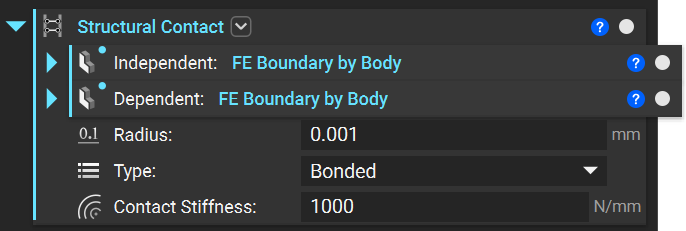
A Structural Contact is an elastic connection between the two models that allow relative motion with a defined stiffness. It’s usually used if you have two surfaces glued together with some material that has a vastly different stiffness than the connected surfaces, which allows the connected surfaces to not move entirely in sync but have specific resistance between them. It’s often used to calculate contact failure and to model connected/welded surfaces more accurately, but generally for any connection dictated by a finite stiffness.
The Type input has two options: Bonded and No Separation
- Bonded: Prohibits relative displacement in the normal and tangential direction
- No Separation: Prohibits relative displacement in the normal direction and allows displacement in the tangential direction
The setup of the Structural Contact is very similar to the setup of a Tie Constraint, but now we define the contact stiffness.
Tip:
We recommend a contact stiffness of 0.5 * (Young’s Modulus of Part 1 + Young’s Modulus of Part 2). Another method of determining the contact stiffness is k = E * A/d (where A is the contact area and d is the contact layer thickness).
Cyclic Symmetry (Beta)
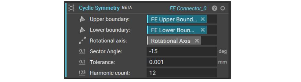
The Cyclic Symmetry block creates tie constraints between an FE Mesh’s upper and lower boundaries. To reduce file size and drastically reduce the run time for parts exhibiting cyclic symmetry, a single sector can be used to assume consistent results for all identical segments of the revolved feature. Currently, the Cyclic Symmetry block only works with parts that do not contact the axis of revolution.
Tip:
Although it is unnecessary, you can create a conformal mesh between the upper and lower boundaries of the sector using the Remesh Surface with Cyclic Symmetry (Beta) block. In some cases, this will yield more accurate results.
Spring
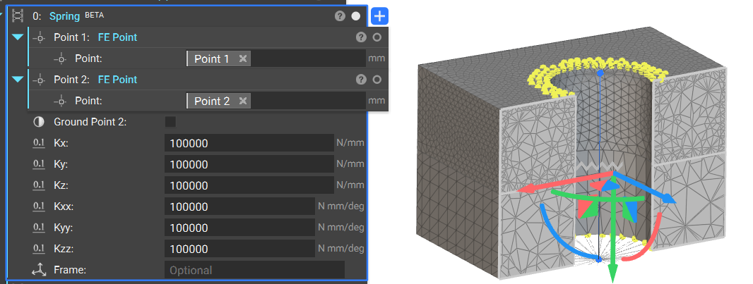
The Spring block creates a spring element between two FE Points. The Spring force is calculated using the following formula:
F = K*(u2-u1)
where:
K = stiffness tensor constructed from the stiffness inputs Kx, Ky, Kz, Kxx, Kyy, and Kzz
u = displacement at a point, which includes both translational and rotational components
Rigid Connector
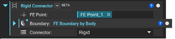
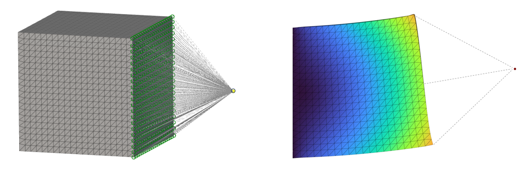
The Rigid Connector block can be used to define a connection between a point and the surface of a domain in a simulation or optimization study. This is typically used in multi-domain simulations where only the mass of the auxiliary domains affects the analysis, while the geometry of these domains can be neglected. These auxiliary domains are modeled as a Solid Domains of FE Points in nTop. This can be used to reduce the size of the finite element model, improving the simulation or optimization solver’s performance without compromising the results’ accuracy.
The Connector input defines the behavior of the nodes on the boundary linked to the motion of the point. It has two options:
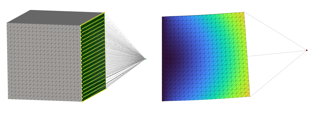
Rigid: The rigid option constrains the nodes on the boundary to move with the point. It prevents relative motion between the nodes on the boundary and behaves like a rigid entity. This is popularly known as the RBE2 connector that connects an independent node (green) to a set of dependent nodes (yellow)
Flexible: This flexible option links the motion of the point to the nodes on the boundary and enables relative motion between these nodes. This distributes the mass between the nodes on the boundary and avoids locally stiffening the model (unlike the Rigid connector). This is popularly known as the RBE3 connector that connects a dependent node (yellow) to a set of independent nodes (green)