

Objective:
Learn how to utilize imported CFD data in nTop to help minimize turbulence within a fluid domain, generate plumbing geometries with near equivalent exit flowrates, or any number of design considerations and performance requirements driven by your CFD. The goal is to utilize CFD early in the design process.Applies to:
- CFD Data
- Plumbing Geometries
- Field Driven Design
Choosing the right CB version:
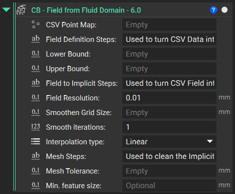
Currently, there are two versions of the Field from Fluid Domain custom block. The complete list of differences between versions 6.0 and 6.1 is described below. Field from Fluid Domain Version 6.0- Performs base field from fluid domain operation
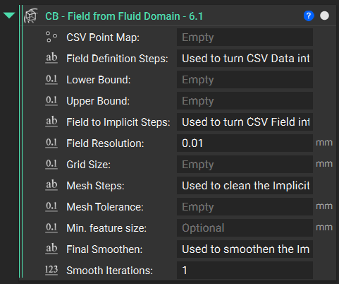
 Field from Fluid Domain Version 6.1
- Performs base field from fluid domain operation
- Smoothen Grid Size input has been changed to Grid Size. This input now controls the Grid Size for both the Smoothen Field and Smoothen Body blocks.
- Smooth Iterations controls both the Smoothen Field and Smoothen Body blocks
- Interpolation Type has been removed and is set to Linear
Block Process:
This section explains what is happening inside the custom blocks to produce the end result. For this example, we will be using Field from Fluid Domain Version 6.1. We use an imported three-dimensional velocity field from CFD results in this example. We truncate the low-velocity regions (i.e., where we may see eddies develop, have areas of low pressure, etc.) and generate a new implicit body from the truncated data. Any variable exported from your CFD tools in CSV format, either as scalar or vector point maps, can be used. 1. Field from Point Map In this step, we turn the point map into a Field. Add a Field from Point Map block, and drag the Import Scalar Point Map block from Step 1 into the first input. From Version 5.0 and on, the Interpolation and Extrapolation were removed from the inputs section. For most cases, Interpolation and Extrapolation will remain the same; therefore, they are now predefined variables. These variables can still be changed when editing the custom block if necessary. Learn more about Interpolation and Extrapolation here.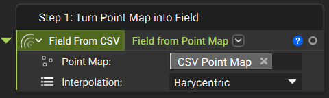 2. Clamp and Ramp the Field
This cuts off the field outside the point list and lets us set all positive space (i.e., outside the part) as 0.
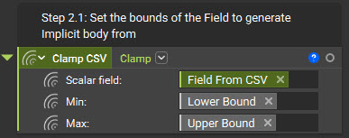
2.1. Using a Clamp block, drag and drop the block from Step 1 into the Scalar field. From what we determined with the HUD, set the Lower and Upper bounds.
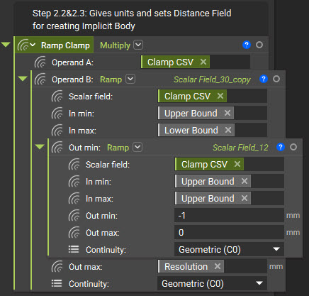
2.2. Using two Ramp blocks, set the positive space. Drag in the Original Body or whichever iteration of your design proceeds this step. Use the Upper Bound for the In min and the Lower Bound for the In Max. The Out max will be the resolution you specified, and the Continuity will be Geometric. The Out min will contain the second Ramp block. The Scalar field is again the Original Body, while the Upper Bound variable is both the In min and max. Set the Out min and Out max values to -1 and 0, respectively. The Continuity should be set to geometric.
2.3. The final sub-step is to multiply these two blocks using the Multiply block.
2. Clamp and Ramp the Field
This cuts off the field outside the point list and lets us set all positive space (i.e., outside the part) as 0.
2.1. Using a Clamp block, drag and drop the block from Step 1 into the Scalar field. From what we determined with the HUD, set the Lower and Upper bounds.
2.2. Using two Ramp blocks, set the positive space. Drag in the Original Body or whichever iteration of your design proceeds this step. Use the Upper Bound for the In min and the Lower Bound for the In Max. The Out max will be the resolution you specified, and the Continuity will be Geometric. The Out min will contain the second Ramp block. The Scalar field is again the Original Body, while the Upper Bound variable is both the In min and max. Set the Out min and Out max values to -1 and 0, respectively. The Continuity should be set to geometric.
2.3. The final sub-step is to multiply these two blocks using the Multiply block.
 3. Bounding Box
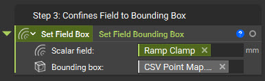
Define the bounding box for the Implicit Body. Utilizing the Set Field Bounding Box block, we insert the block from Step 2.3 and the bounding box of the original imported point map.
3. Bounding Box
Define the bounding box for the Implicit Body. Utilizing the Set Field Bounding Box block, we insert the block from Step 2.3 and the bounding box of the original imported point map.
 4. Smoothen the Field
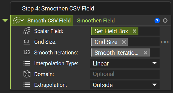
Our next step is to smooth out the Field and generate our Implicit. This is done by utilizing the Smoothen Body block. The first input is the block from Step 3. It is a matter of adjusting the Grid Size and Smooth Iterations as needed. Depending on the size of our part, the density of the imported points (i.e., mesh density form analysis) means the Grid Size especially may vary. The Smooth Iterations/Interpolation types have been removed and are now predefined variables.
4. Smoothen the Field
Our next step is to smooth out the Field and generate our Implicit. This is done by utilizing the Smoothen Body block. The first input is the block from Step 3. It is a matter of adjusting the Grid Size and Smooth Iterations as needed. Depending on the size of our part, the density of the imported points (i.e., mesh density form analysis) means the Grid Size especially may vary. The Smooth Iterations/Interpolation types have been removed and are now predefined variables.
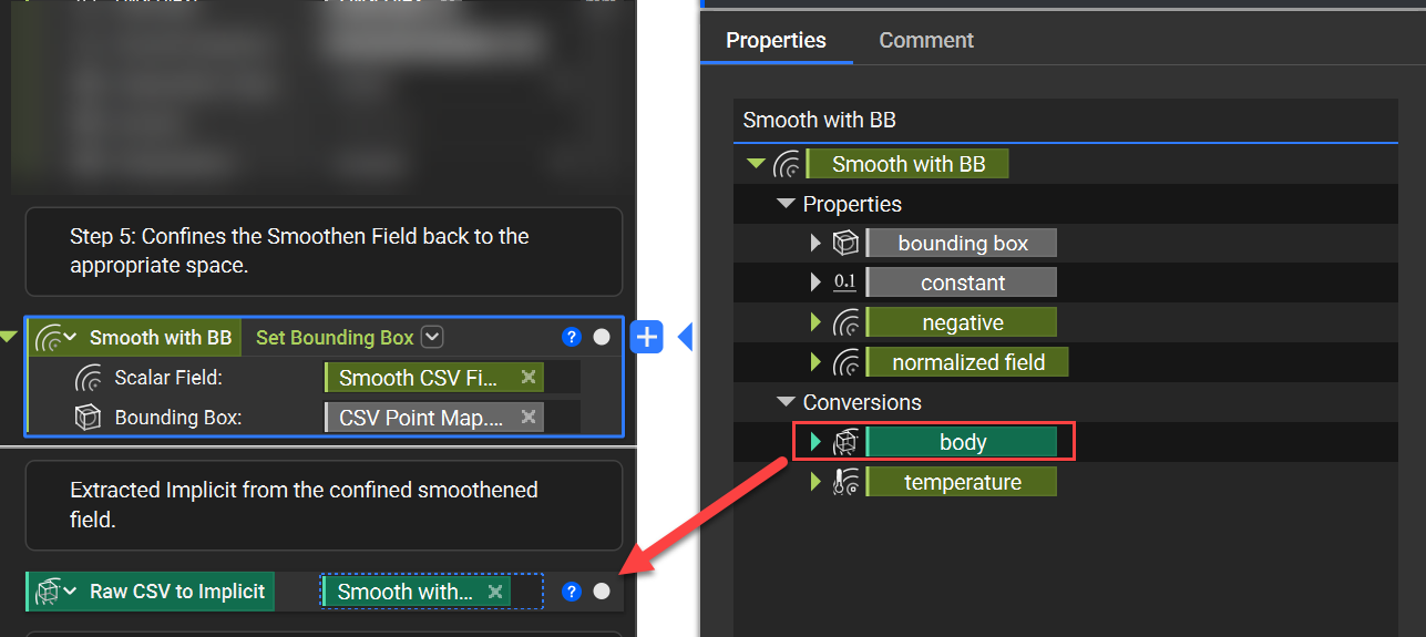
 5. Reapplying the Bounding Box and Extracting the Implicit Body
The resulting field of the Smoothen Field block is larger than our CSV bounding box. To contain the field, we can use another Set Bounding Box block.
5. Reapplying the Bounding Box and Extracting the Implicit Body
The resulting field of the Smoothen Field block is larger than our CSV bounding box. To contain the field, we can use another Set Bounding Box block.
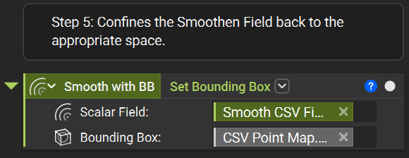 We then extract the Implicit Body property chip from the properties panel of the Smooth with BB variable.
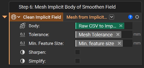
 6. Meshing for a Cleaner Implicit
The following step is to use a Mesh from Implicit Body block with our raw implicit from Step 5. This will allow us to apply the Tolerance and Minimum Feature Size inputs. The resulting mesh will be a cleaner result.
6. Meshing for a Cleaner Implicit
The following step is to use a Mesh from Implicit Body block with our raw implicit from Step 5. This will allow us to apply the Tolerance and Minimum Feature Size inputs. The resulting mesh will be a cleaner result.
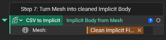
 7. Resulting Implicit
The second to last step of the custom block is to convert the polished mesh into an implicit body.
7. Resulting Implicit
The second to last step of the custom block is to convert the polished mesh into an implicit body.
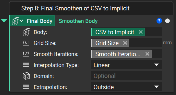
 8. Final Smoothen
The final step is to smoothen the implicit body.
8. Final Smoothen
The final step is to smoothen the implicit body.
 Post-Processing
Additional steps can be taken to generate the ‘final’ implicit, of our fluid domain, either for our next iteration or to begin creating the piping geometry we intended to manufacture.
The first thing we typically need to do is Boolean Intersect our block from Step 6 with the Original design space; during the truncation and smooth process, our Inlet and Outlets ports can get distorted. The Boolean Intersect step trims them off, and then we Boolean Union the intersected body to our desired inlet and outlet ports; see Image #2 below.
Post-Processing
Additional steps can be taken to generate the ‘final’ implicit, of our fluid domain, either for our next iteration or to begin creating the piping geometry we intended to manufacture.
The first thing we typically need to do is Boolean Intersect our block from Step 6 with the Original design space; during the truncation and smooth process, our Inlet and Outlets ports can get distorted. The Boolean Intersect step trims them off, and then we Boolean Union the intersected body to our desired inlet and outlet ports; see Image #2 below.
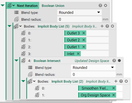 Image #1: Boolean Operations to clean and generate final geometry.
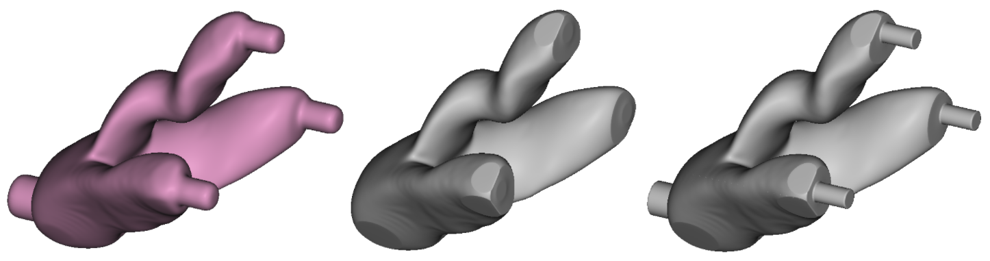 Image #2: The image on the left is the output from Step 6 (Smoothen Body), the image in the center is the intersection with the original design space (trimming the ports and re-confining to design space), the image on the right is the ‘final’ geometry.
Now that you have your final implicit model with the appropriate ports, our next steps are to mesh the implicit, evaluate how this iteration compares to the performance requirements, and either repeat the iterative process (i.e., the procedure above) or begin shelling operations of the fluid domain created above to generate the plumbing geometry we would eventually manufacture.
Image #3 below shows the iterations and results from the case study presented in this article. Beginning with an oversized design space (the top left part) and defining the constraint to have Outlet Uniformity with one inlet and three outlets. After only four iterations, the part and process converged on a solution resulting in the three outlets within 3.5% of the mean exit flowrate.
Image #2: The image on the left is the output from Step 6 (Smoothen Body), the image in the center is the intersection with the original design space (trimming the ports and re-confining to design space), the image on the right is the ‘final’ geometry.
Now that you have your final implicit model with the appropriate ports, our next steps are to mesh the implicit, evaluate how this iteration compares to the performance requirements, and either repeat the iterative process (i.e., the procedure above) or begin shelling operations of the fluid domain created above to generate the plumbing geometry we would eventually manufacture.
Image #3 below shows the iterations and results from the case study presented in this article. Beginning with an oversized design space (the top left part) and defining the constraint to have Outlet Uniformity with one inlet and three outlets. After only four iterations, the part and process converged on a solution resulting in the three outlets within 3.5% of the mean exit flowrate.
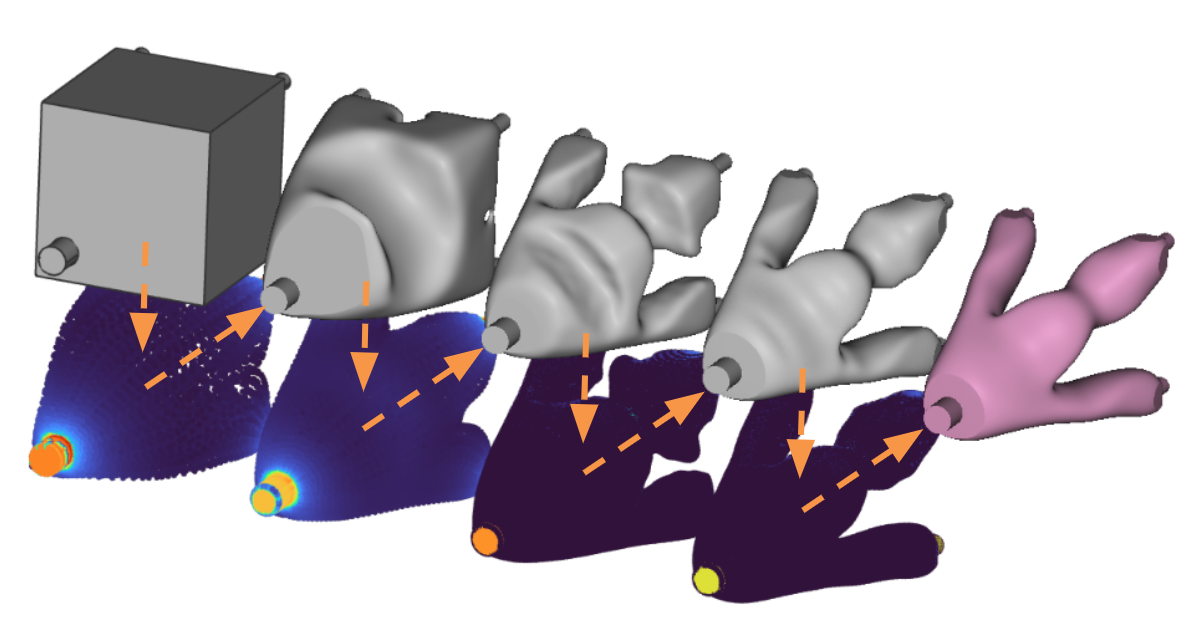
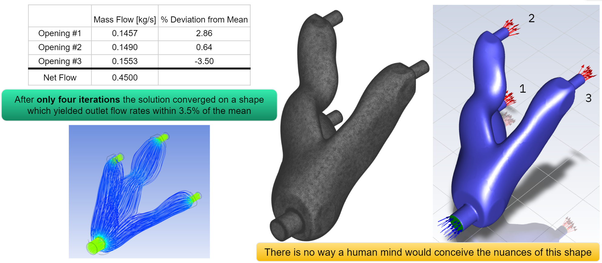 Image #3: The top half of the image shows the iterations and velocity fields brought in from Ansys Fluent. The bottom half of the images show the final iterations’ results (the pink part seen above).
If you still have questions, the support team would be happy to help you.
Image #3: The top half of the image shows the iterations and velocity fields brought in from Ansys Fluent. The bottom half of the images show the final iterations’ results (the pink part seen above).
If you still have questions, the support team would be happy to help you.