Objective:
Learn how to use Boundary Conditions in a Static Analysis. Boundary Conditions (BCs) can be thought of as the environment your part is in. They include Forces, Displacement Restraints, Heat Generation, Pressure, and more. All of the internal and external elements acting on your model. You need a minimum of two BCs to run a simulation. The image below shows the current options for solid simulations on the left, and options for fluid simulations on the right.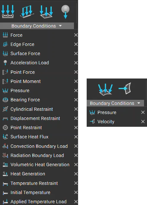
Procedure: Static Analysis BC
Looking at the Brake Pedal example, we can identify what BCs we want to use in our Static Analysis. The force is where your foot would be pressing on and the displacement restraint is where the pedal is connected to another piece and fixed in place. A Displacement Restraint is usually required when forces are involved to ensure the part is fixed in space. Without it, the simulation wouldn’t be able to run.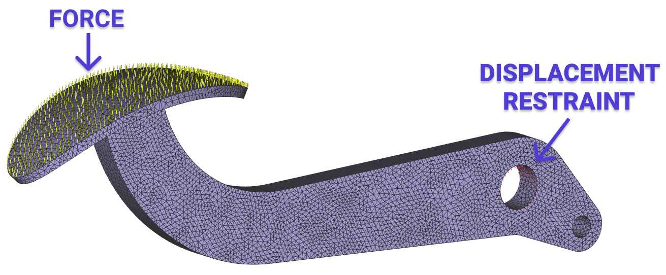
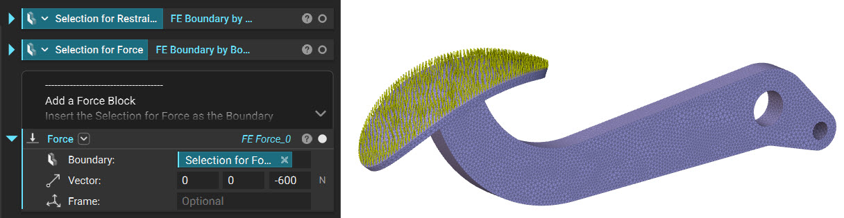
1. Create a Force BC:
- Add a Force block to the workflow
- Insert the FE Boundary by Body into the Boundary input
- Set the Vector to (0,0,-600N). This represents a foot acting on the brake pedal head with a factor of safety.
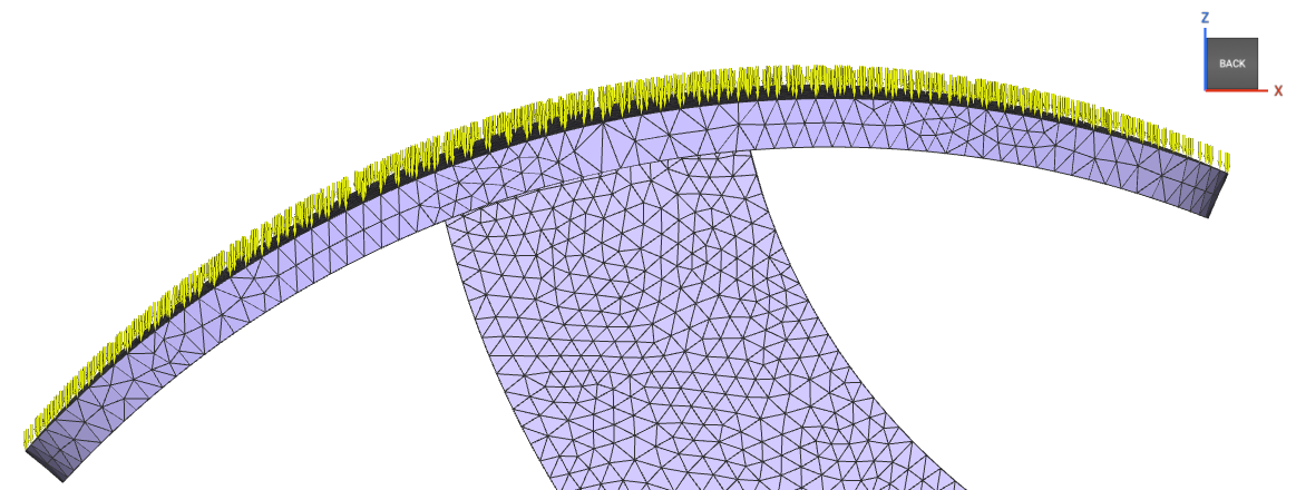 The downward arrows represent the -600N of Force acting in the negative Z-direction over the entire brake pedal head. If you want more control over the direction of the force, you can edit it using the ‘Frame’ input.
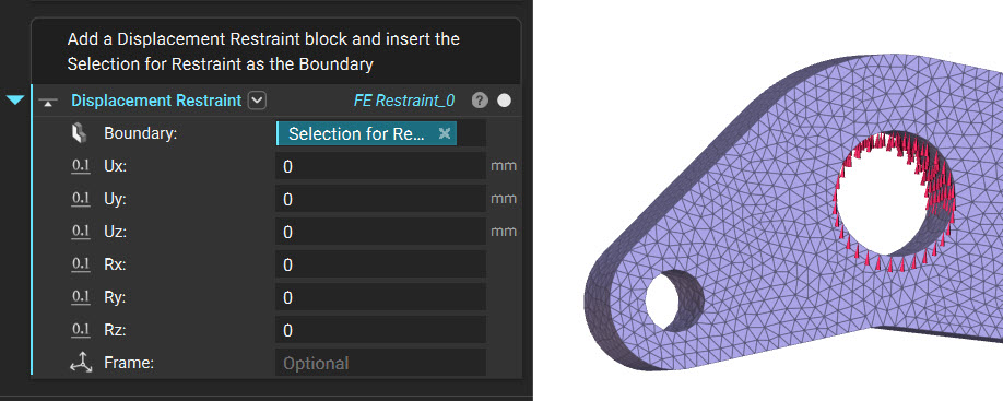
2. Create a Displacement Restraint BC:
The downward arrows represent the -600N of Force acting in the negative Z-direction over the entire brake pedal head. If you want more control over the direction of the force, you can edit it using the ‘Frame’ input.
2. Create a Displacement Restraint BC:
- Add a Displacement Restraint block
- Insert the FE Boundary by Flood Fill selection into the Boundary input
Procedure: Fluid Analysis BC
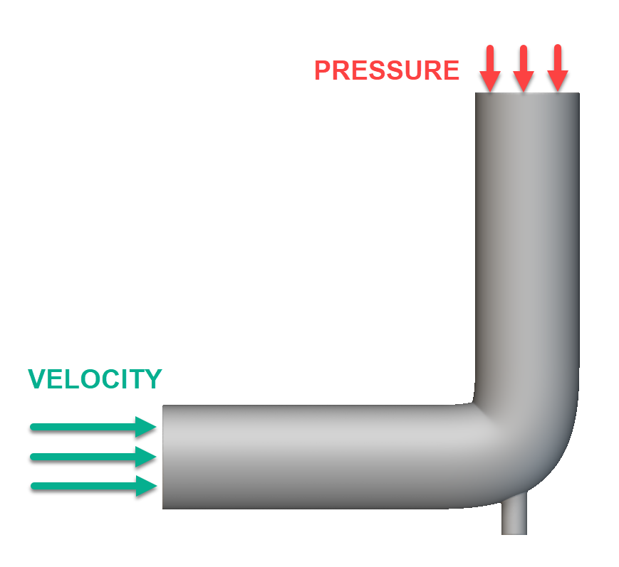 In this pipe example, we want to apply an intake velocity for a fluid. We need to have a second boundary condition applied for the simulation to run, so we will specify a pressure with no magnitude at the other end of the pipe.
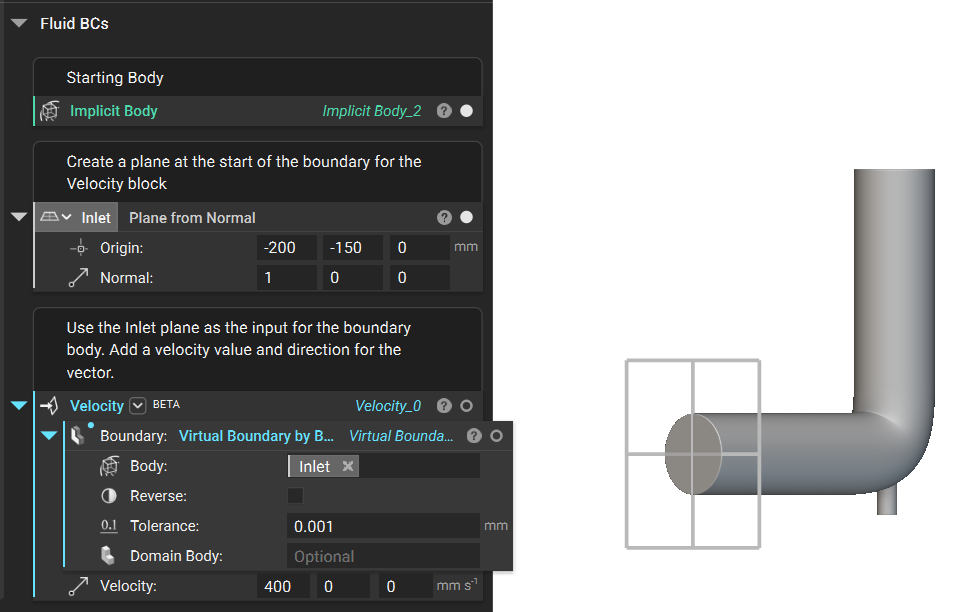
1. Create a Velocity BC:
In this pipe example, we want to apply an intake velocity for a fluid. We need to have a second boundary condition applied for the simulation to run, so we will specify a pressure with no magnitude at the other end of the pipe.
1. Create a Velocity BC:
- Add a Plane from Normalblock and position it at the center of the intake surface. Ensure the normal direction is directed towards the body.
- Add a Virtual Boundary by Body block. Insert the plane into the Body input.
- Add a Velocityblock. Insert the Virtual Boundary by Bodyblock into the Boundary input. Insert a value of 400 mm/s into the X input box of the Velocity input.
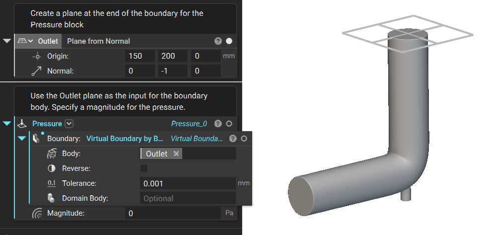
 2. Create a Pressure BC:
- Add a Plane from Normalblock and position it at the center of the outlet surface. Ensure the normal direction is directed towards the body.
- Add a Virtual Boundary by Body block. Insert the plane into the Body input.
- Add a Pressureblock. Insert the Virtual Boundary by Bodyblock into the Boundary input. Insert a value of 0 Pa into the Magnitude input
 And that’s it! You’ve successfully added boundary conditions to your part.
Are you still having issues? Contact the support team, and we’ll be happy to help!
And that’s it! You’ve successfully added boundary conditions to your part.
Are you still having issues? Contact the support team, and we’ll be happy to help!