Parametric Primitives & Math Blocks

​

Creating Geometry from Primitives

Before we learn how to incorporate parameterization, we first need to understand how to create basic geometry in nTop. You can find standard 2D and 3D shapes in the nTop Ribbon under the Create tab. From the Create tab, you can select the drop-down menu under Primitives to see the available shapes.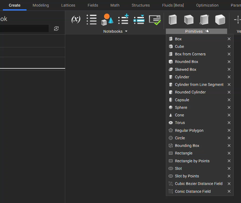 The Primitives tab is located in the Create tab of the Ribbon Once you select a shape from the list, the block inserts into your notebook. Then you can modify the block’s inputs to change the location, size, etc. of the shape. You can specify new input values by entering them in the box next to the input or by dragging the bidirectional arrow that appears next to the box. Please keep in mind that the bidirectional arrow will only appear for certain scalar input values, not for every input. An example of adding Primitives to the Notebook using the Ribbon Despite both the Box and Circle blocks being Primitives, they have different block types. The Box is an Implicit Body while the Circle is a Profile. You can determine a block’s type by hovering over the icon next to its name. Now that we know how to insert Primitives, we need to understand how they can interact with each other.

​

Variables and Properties

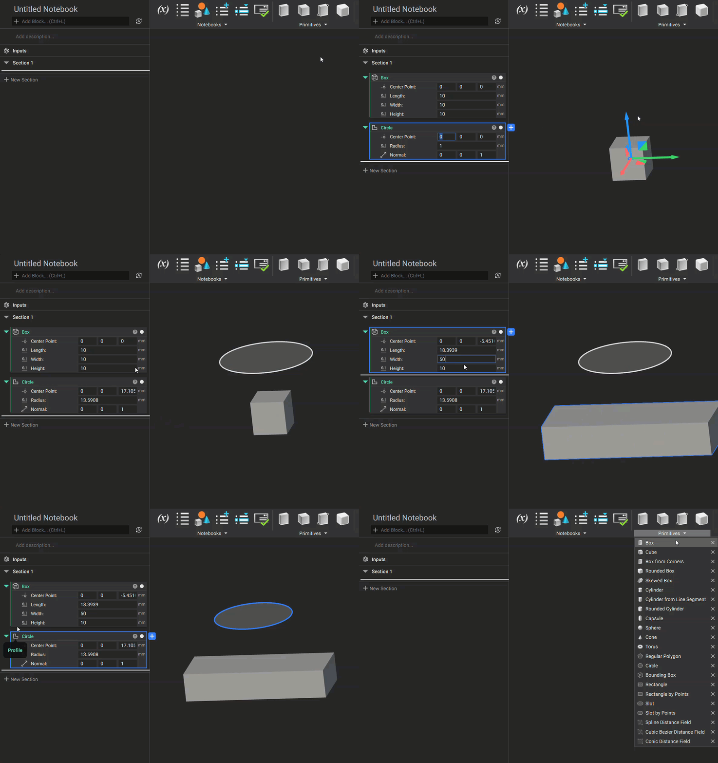
Variables are the key to keeping a tidy Notebook. You can turn any block or input into a variable, allowing easy access, reference, and manipulation. Once you make it a variable, the block or input remains in your Notebook. The variable is represented as a simple chip when used in other blocks. Use variables to drive your workflow with key parameters and streamline your design process. As a best practice, we recommend using variables whenever possible to keep your notebook organized.

​

Parameterization using Variables and Properties

In nTop, parameterization means encoding your design intent as variables and parameters that drive geometry, rather than defining static shapes. Instead of modeling a fixed part, you build a workflow where inputs (dimensions, positions, etc.) are exposed as variables — so changing a single value automatically updates the entire design. This enables rapid iteration, optimization, and automation across many configurations without manually rebuilding geometry. The GIF below shows an example of creating a parameterized capsule. The Cylinder Radius input is converted to a variable so that it can be used to define the Radius of the Sphere blocks. Next, the Start and End Point property chips are extracted from the Cylinder, and are used to define the Center Point inputs of the Sphere blocks. Using a Boolean Union, we can combine the three implicit bodies into a single body.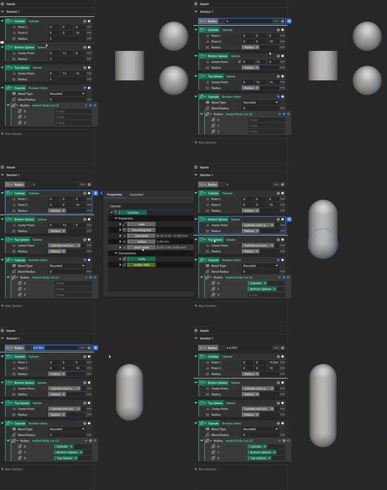 An example using a Cylinder and Spheres to create a parametric Capsule body The result is a parameterized capsule that is able to adapt its shape when we change the input values.

​

Datum/Reference Geometry

Another useful parameterization strategy is to build your geometry in reference to datums (Points, Planes, Axes, Frames, etc.). By creating one or more datums, you can parameterize your geometry without having to hard-code coordinate values. This lets the geometry adapt to any changes made to the datum. In the example below, a Spline through Points block is generated using the Plane’s origin x-coordinate value. This ensures the Spline remains aligned with the plane even if the Plane’s Origin location changes.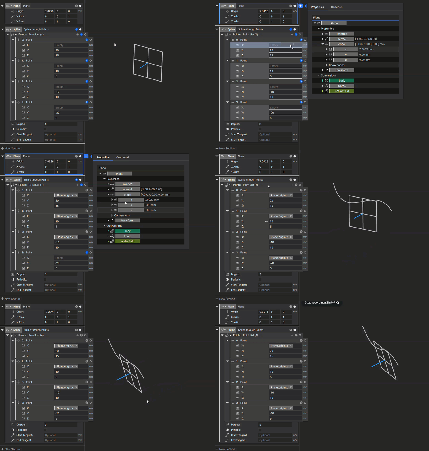 Using X coordinate property of the Plane’s origin to define a Spline through Points

​

Visualizing Implicit Bodies

​

Bounding Boxes

As discussed in previous sections, Implicit Bodies are equation models comprised of Signed Distance Fields. But how do we go from looking at a field in the field viewer to a 3D implicit body? Most times we can use what’s called a Bounding Box. A Bounding Box is a 3D box that represents the overall dimensions of a scalar field or implicit body. It is defined by two corner points at the maximum and minimum of your geometry’s span. The Bounding Box is the limit of the geometry, so anything that extends beyond the box will be removed from the output body/field. When working with fields and implicit bodies, nTop will attempt to automatically apply an appropriately sized Bounding Box. But there are situations (like working with infinite or unbounded fields) where users will need to manually apply a Bounding Box in order to properly define an output field/body. As an example, we can show how to create a solid body from a scalar field. The equation below represents a gyroid field: sin(x)*cos(y) + sin(y)*cos(z) + sin(z)*cos(x) After entering this equation into nTop, we can use the Field Viewer to visualize the gyroid field.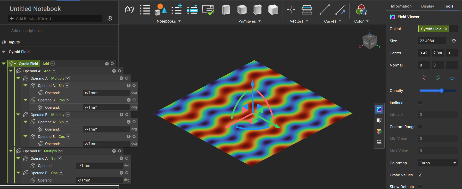 An infinite gyroid field created using the gyroid equation The Gyroid shape is created using Sin and Cos. These operations require the units to be in degrees, not length. Therefore, we can divide each value by 1mm to remove the length units; otherwise, the block will error out.

​

Set Bounding Box

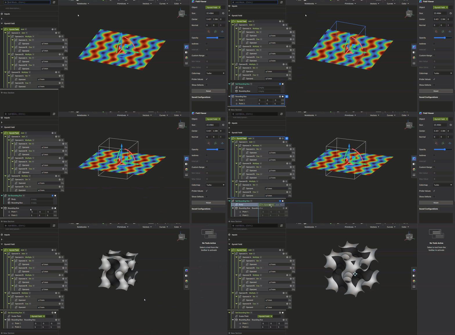
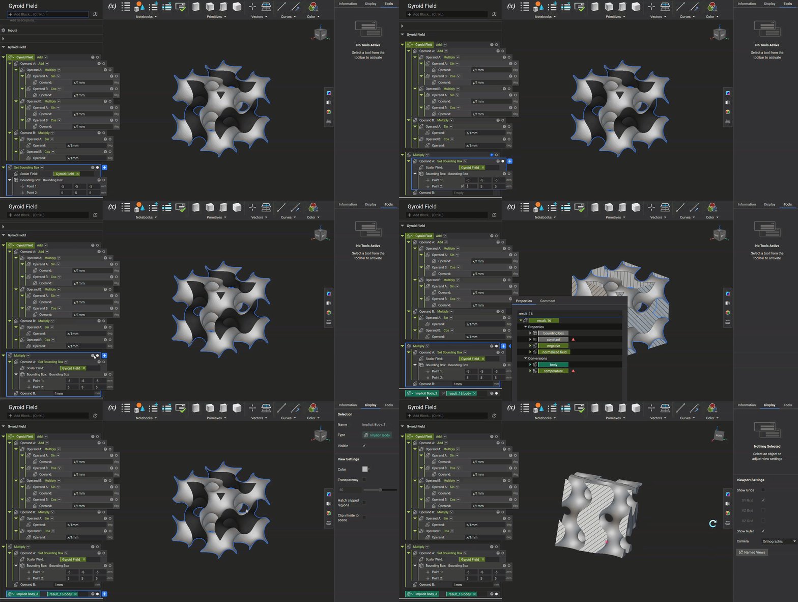
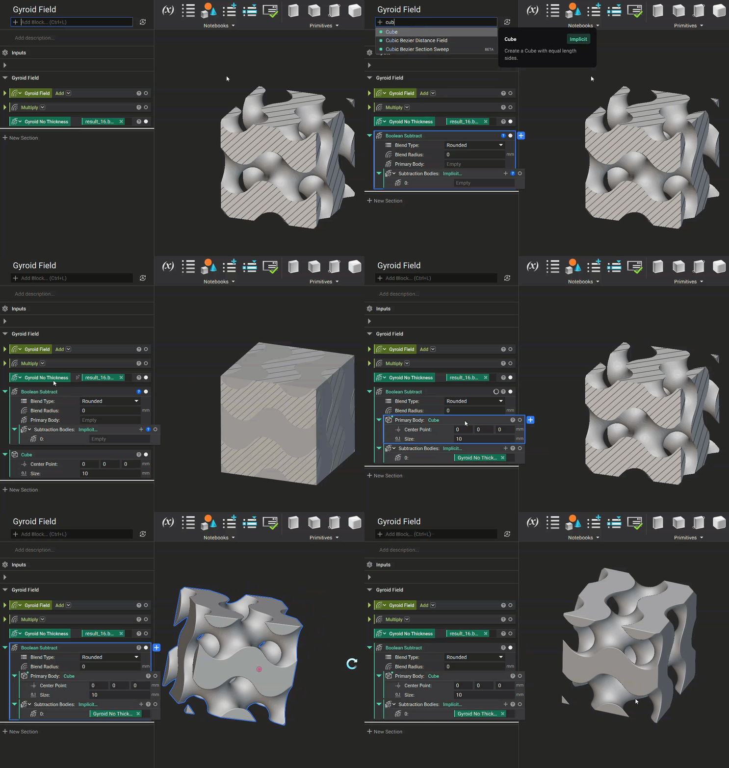
Now that we have our field, we need to apply a Bounding Box to define the bounds of the geometry. By adding a Bounding Box and a Set Bounding Box block to our notebook, we can visualize the gyroid surface. Using the Set Bounding Box block to visualize the zero-thickness gyroid contained within the Bounding Box This surface is not an implicit body yet, as we removed the units to generate the gyroid field. To fix this, we can multiply the gyroid surface by 1mm to reapply the units. Finally, we extract the implicit body from the properties panel. The result is a zero-thickness gyroid cube. The end of the gif below also shows how you can enable hatching to represent clipped regions of your design. Clipped regions are areas within your bounding box that lack physical geometry. Applying units to the gyroid field using a Multiply block. The gyroid implicit is then extracted from the properties panel of the field If we wanted to create a solid implicit body using the zero-thickness gyroid, the easiest method is to subtract the gyroid from an existing solid body. Using a Boolean Subtract block, we can subtract the gyroid from a Cube to create a thickened gyroid body. Using a Boolean Subtract block, we can create a solid body Gyroid

​

Refine Bounding Box

There are instances where nTop will attempt to apply an appropriately sized Bounding Box, but the result may be larger than the implicit body. This can lead to downstream issues if nTop thinks a body is much larger than it actually is. The solution for these scenarios is to use the Refine Bounding Box block. Using an input Body and Grid Size, nTop will recalculate the Bounding Box size. The gif below shows an example using a cube with a very oversized bounding box. After refining the bounding box, the result is very close to the geometry’s surface. A smaller grid size will create a more conformal box, but may take longer to calculate.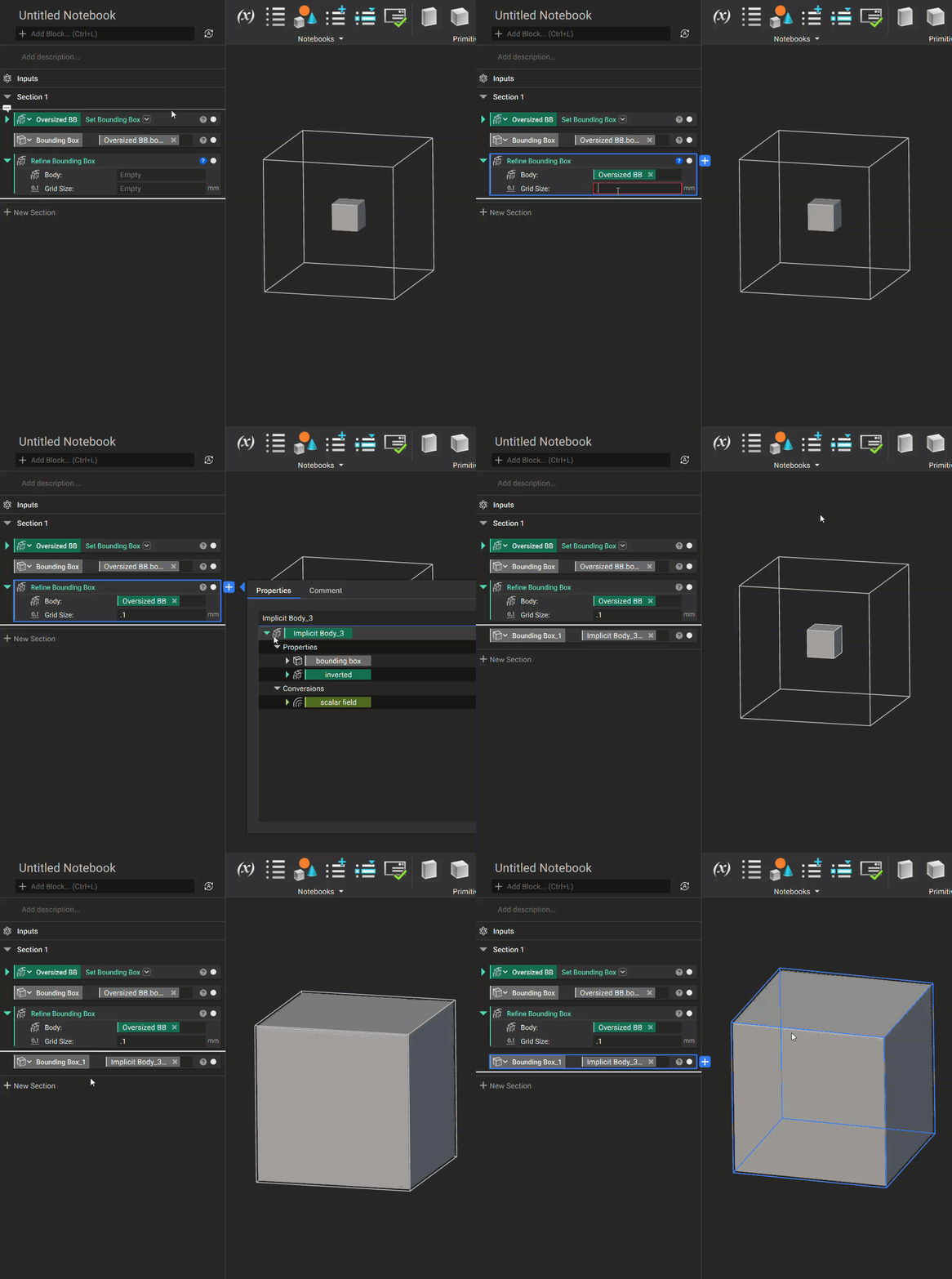 Using the Refine Bounding Box block to create a more size accurate Bounding Box for the Cube

​

What to Take Away:

• Boolean Operations are the core utility for implicit bodies. Most workflows utilize these blocks to modify implicits.
• Block & Input variables help you stay organized in the notebook. nTop notebooks can get confusing when blocks are consistently nested inside one another. Variables reduce clutter by reducing nested blocks and using helpful names.
• Parameterization keeps geometry connected and allows for quick iterations. Parameterizing your workflow lets you create unbreakable geometry connected through property and input variables. Modifying parameterized variable values lets the geometry quickly recalculate and generate new geometry.
• Bounding Boxes are the key element in visualizing geometry. Bounding boxes define the maximum and minimum boundaries of a scalar field or implicit body. Anything outside of these bounds will not be visualized.

​

What’s Next

You now have an understanding of how to create basic geometry, create block and property variables, parameterize your workflow, and visualize implicit bodies. The next lesson will broaden your understanding of nTop’s modeling and creation tools using splines, curves, and profiles.