

- Explain how a field contains more information than whether a point is inside or outside a body.
- Describe how a field extends infinitely through space, beyond the implicit body it represents.
- Distinguish between the field itself and its on-screen visualization.
- Explain how union, subtract, and intersect combine multiple fields through arithmetic Boolean operations—and why they behave differently in nTop than in traditional CAD.
Signed Distance Fields
A signed distance field (SDF) is a function (i.e. f(x,y,z)) that assigns a value to every point in 3D space based on its distance from the nearest surface of a body and whether the point lies inside or outside that body. As introduced in Lesson 1, the sign indicates the point’s position relative to the surface:- Negative — the point is inside the body
- Positive — the point is outside the body
- Zero — the point lies exactly on the surface
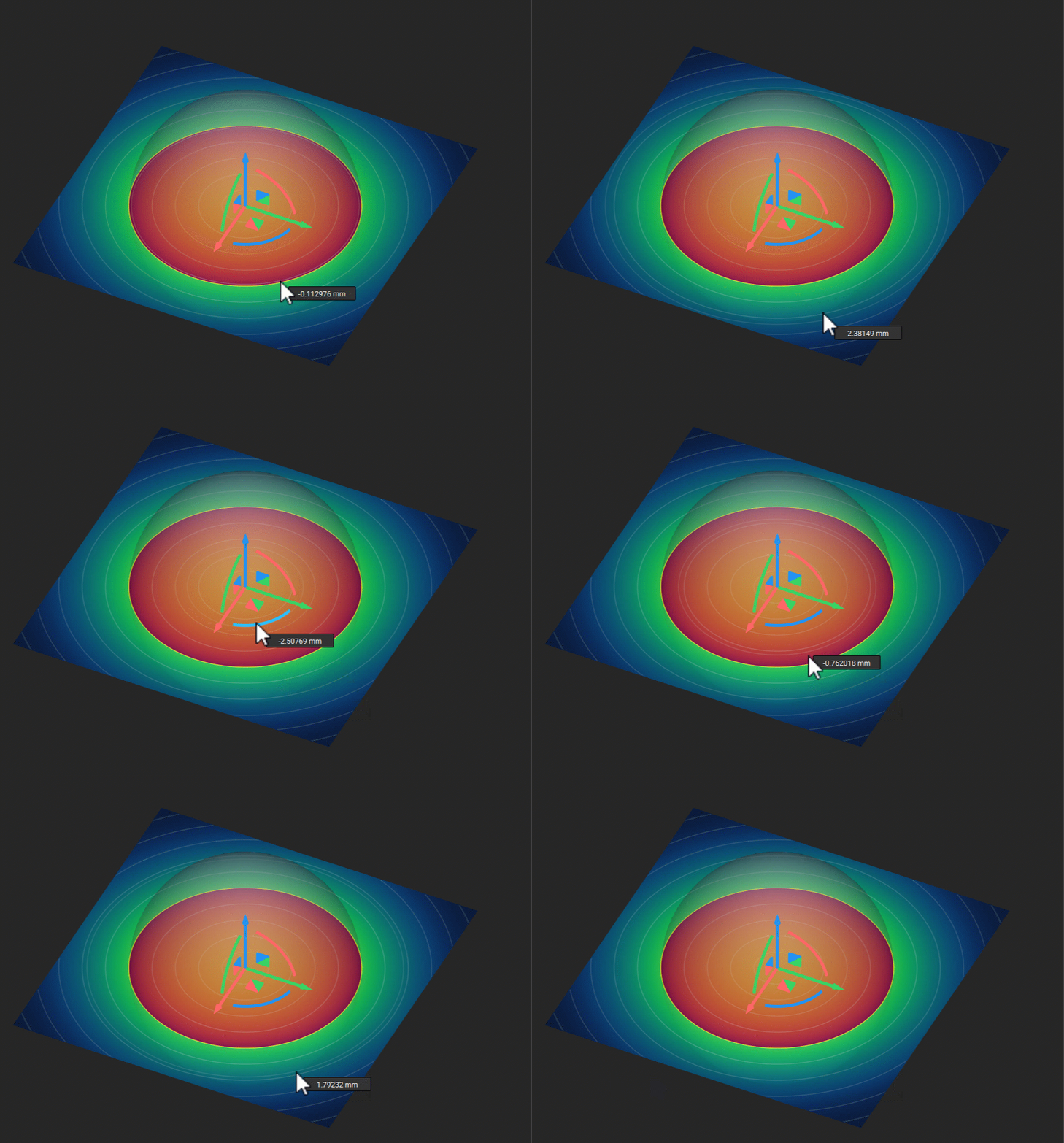
Isosurfaces
If the body’s surface is defined by the points where the field value equals zero, then any other constant field value also defines a surface. For example, all points where the field equals −1 mm form one surface, while all points where it equals 2 mm form another. These constant-value surfaces are called isosurfaces. Together, they form nested surfaces inside and outside the body, like the layers of an onion. The lines shown in the GIF above represent these isosurfaces for the Field of a Primitive Sphere, with each line corresponding to a constant field value. This concept underpins many implicit modeling operations you will encounter later. Offsetting a body does not require constructing a new surface; instead, the operation shifts which field value defines the body’s boundary. Shelling uses the region between two isosurfaces to define the shell. Similarly, applying a blend radius to a Boolean operation modifies how the underlying fields combine near the resulting surface.Why Distance Matters, Not Just Sign
Any function that is negative inside a shape and positive outside will describe that shape correctly. It will not necessarily be a signed distance field. The distinction matters because the operations above depend on the magnitude being a true distance. If the field says −1 at a point that is actually 4 mm inside the body, an offset driven by that field will land in the wrong place. A well-behaved SDF has a recognizable signature in the Field Viewer: its isolines run parallel to the surface and are evenly spaced, because moving 1 mm through space changes the field value by 1 mm. Crowded or uneven isolines indicate the field has been distorted and no longer measures true distance. You will use this signature as a diagnostic long before you need the underlying math. Course 2 covers what causes a field to stop being a true SDF, and what to do about it.Fields Extend Beyond Solid Bodies
Fields are not exclusive to closed bodies. Simple geometry carries simple fields: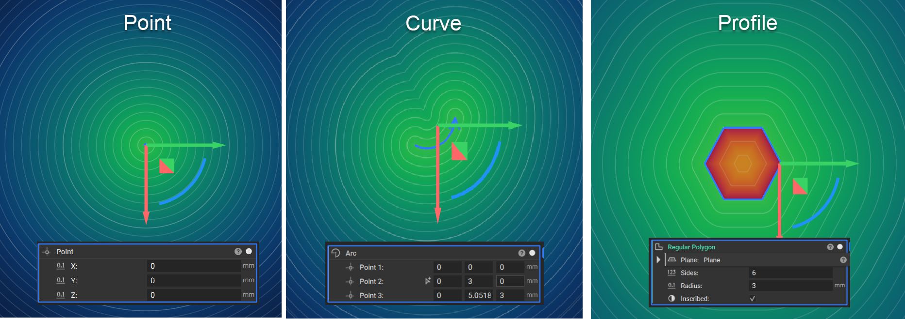
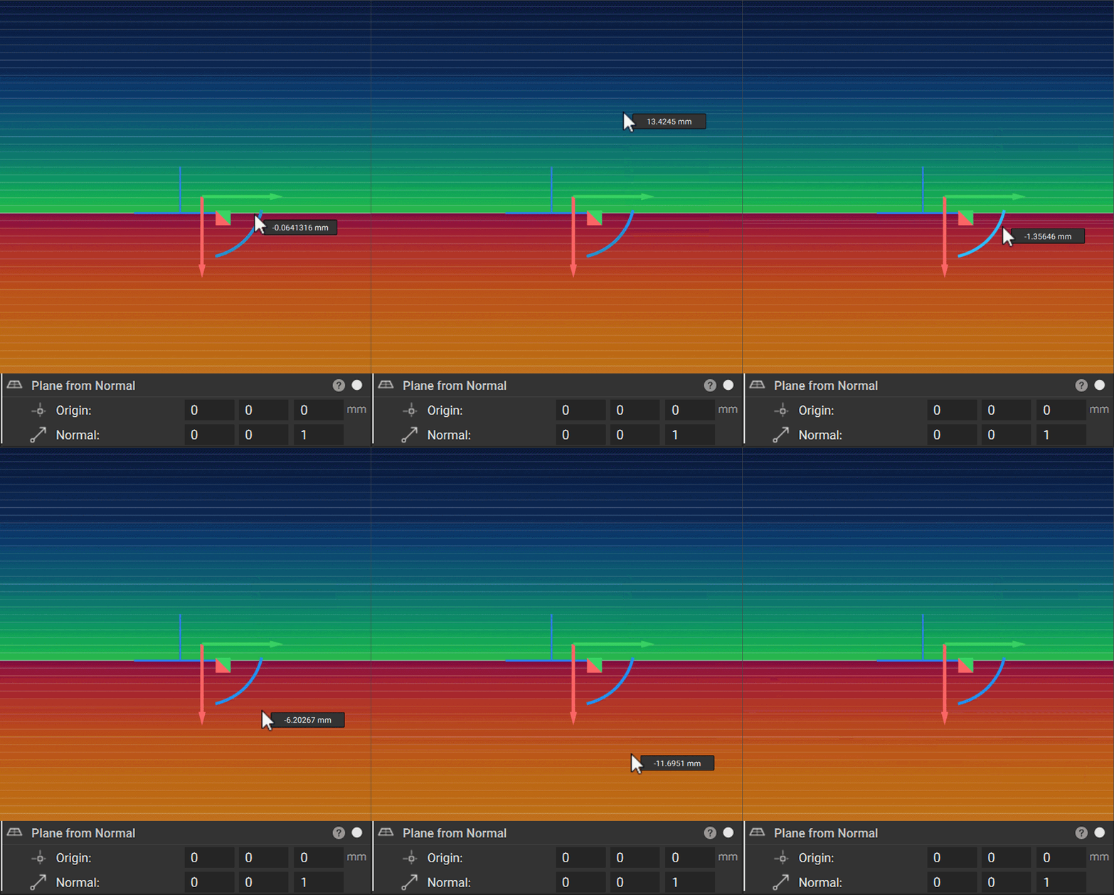
Fields are unbounded
Consider the plane in the table again. Where does its field end? It does not. A plane’s field is defined throughout all of space. Even a point one kilometer away still returns a value representing the signed distance to the plane. The same principle applies to the field of a point, a curve, or a sphere. Fields extend infinitely through space . The geometry itself may occupy a finite region, but the field that describes it does not. This behavior often goes unnoticed because many fields you encounter first contain an enclosed negative region. For a closed body such as a sphere, negative field values define a finite volume that nTop can render as solid geometry. The field continues infinitely beyond the body, but it does not display the positive region as material. Not all fields, however, contain an enclosed negative region:- Plane: Divides space into two infinite half-spaces; neither side is enclosed.
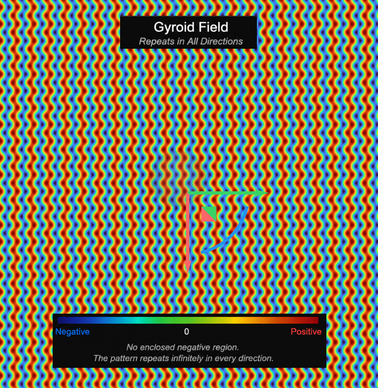
- Triply Periodic Minimal Surface (TPMS) fields: Fields such as gyroid, Schwarz, and diamond repeat indefinitely in all three spatial directions.
- Point and curve distance fields: Remain positive everywhere because a point or curve does not enclose a volume.
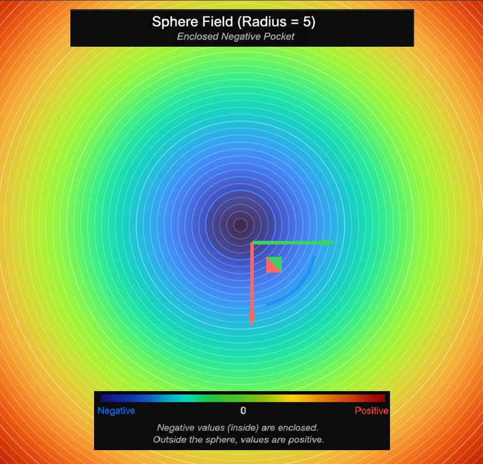
Giving an Unbounded Field an Extent
When you need to visualize or use an unbounded field as geometry, the Set Bounding Box block assigns it a finite region of interest. The underlying field does not change; the bounding box simply defines the portion of the field that nTop evaluates as a body. For example, applying a bounding box to an infinite gyroid field produces a finite gyroid body that you can visualize and use in downstream operations such as Booleans.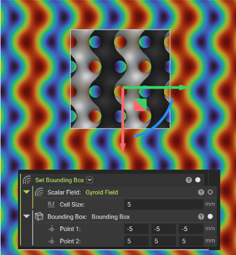
Bounding Boxes Are Estimates
Every implicit body has a Bounding Box property that defines the region containing the body. This box may extend slightly beyond the body’s actual boundaries, which is expected. Because an implicit surface is defined by a field rather than stored explicitly, nTop must determine its extent by searching the field. Computing a perfectly tight bounding box for an arbitrary field can be computationally expensive, so nTop uses a conservative estimate that safely contains the entire body. For a tighter bounding box, use Refine Bounding Box under Utilities in the Modeling tab, or manually use Set Bounding Box with the parameters that control your implicit body. Refine Bounding Box block recomputes the bounding box of an implicit body to a specified tolerance, producing a closer fit around the body’s actual extent. It is particularly useful after operations such as Booleans, where the resulting body’s bounding box may remain larger than the geometry itself.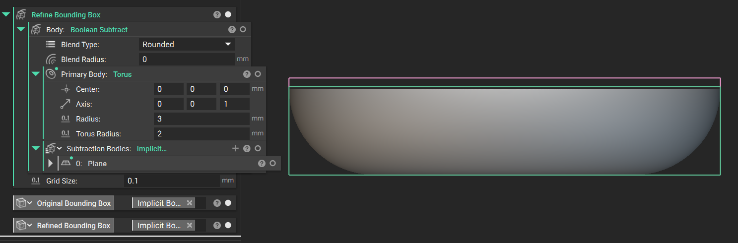
Note: Using Bounding Boxes and the Set Bounding Box block will be covered in the next course
How Fields Generate Geometry
Earlier in this learning path, we introduced a fundamental distinction: CAD stores geometry as faces, edges, and vertices, while nTop stores the function that defines the geometry. The surface is generated where that function equals zero. This distinction has several important implications:- No faces are stored to select or reference, avoiding failures when topology changes or disappears.
- Bodies are watertight by construction because the field continuously defines what is inside and outside.
- Geometric complexity is inexpensive. Adding detail increases mathematical computation, which nTop’s parallel architecture handles efficiently, without introducing the topology or file-size burden associated with the faces and edges of traditional CAD.
The Field and Its Visualization Are Not the Same
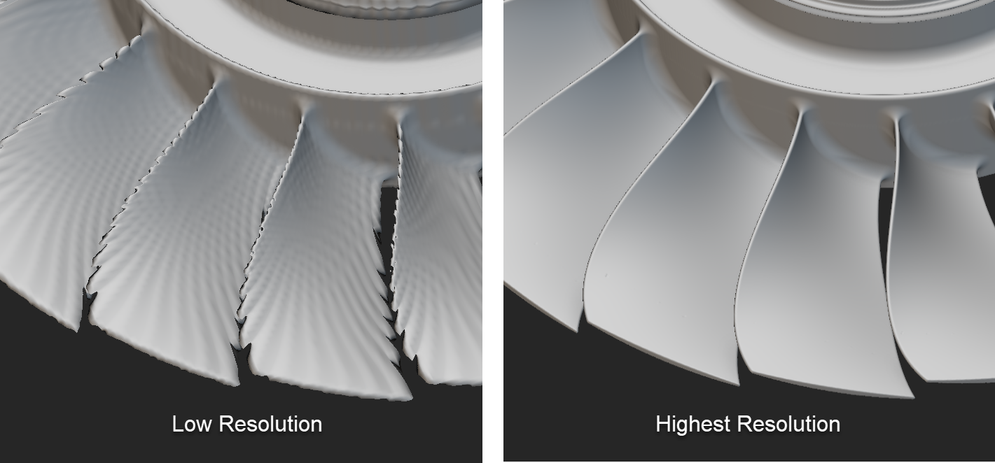
The SDF defines the geometry; the Viewport visualizes it. The field is a continuous function that returns a value at every point in space. The Viewport samples that function and renders the zero surface according to the selected display resolution. Increasing the resolution from Low to Highest improves the visualization, but it does not change the underlying geometry. This distinction has several important implications:- Viewport resolution affects visualization, not geometry. Increasing resolution improves visual fidelity at the cost of render time, but it does not change the underlying implicit body or the quality of geometry exported from it. Use Low or Medium resolution while working and increase it when a closer visual inspection is necessary.
- Visual artifacts do not necessarily indicate incorrect geometry. Thin walls may appear to have holes, lattice beams may look disconnected, and fine repeating features may display artifacts when the Viewport cannot fully resolve their detail. Use Precise Render (Ctrl + H), increase the Viewport resolution, or enable Adaptive Resolution—introduced in the previous lesson—when you need a more accurate visualization.
- When in doubt, probe the field. If the visualization still appears incorrect, use the Field Viewer to inspect the underlying field directly. For example, if a wall appears missing, a negative field value where material is expected confirms the geometry exists—the Viewport is simply not resolving it clearly.
The Field Viewer: Looking at an SDF
The field extends continuously throughout three-dimensional space, so you can’t visualize it all at once. The Field Viewer addresses this by displaying a two-dimensional slice through the field—a window that can be positioned wherever you want to inspect its values. The previous lesson introduced how to access and use the Field Viewer. This section builds on that foundation by exploring its functionality in greater detail.Opening the Field Viewer
With a block selected, press the shortcut key “F”. You can also right-click an object in the Viewport and choose Field Viewer, or open it from the Field Viewer button in the view toolbar. When you open it from a selected block, the Object input is filled in for you. If you open it with nothing selected, the input is empty — type the name of the block whose field you want to inspect.Positioning the window
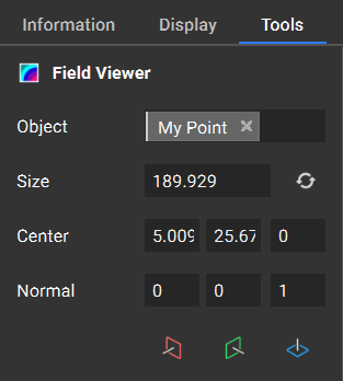
- Size — how large the plane is. Use the reset button beside the input to fit it to the current view.
- Center and Normal — type values directly, or drag the gimbal in the 3D scene.
- Orientation buttons — the YZ, XZ, and XY buttons snap the normal to a global axis. This is the fastest way to compare the same field from three directions.
Reading what you see
- Opacity — Controls the field’s opacity. Drag the slider to adjust its transparency.
- Isolines — white lines connecting points of equal field value, on by default. Leave Interval at 0 for adaptive spacing, or enter a value to fix it. Evenly spaced, surface-parallel isolines are the signature of a healthy SDF. You can toggle this functionality on or off.
- Custom range — clamps the display to a minimum and maximum you choose, giving you fine color resolution in a narrow value band.
- Colormap — Implicit is applied automatically to implicit bodies and is tuned to make the inside/outside boundary legible. Scalar fields default to Turbo; Distance Field is also available.
- Probe Values — Hover anywhere on the plane to view the field value at that point. The corresponding isoline highlights, showing all other points in the slice with the same field value. You can toggle this functionality on or off.
- Show Defects – Highlights field discontinuities as red regions—areas where the field value changes abruptly and may produce artifacts, such as unexpected walls or holes in toolpaths during slicing. You can toggle this functionality on or off.
- Highlight Zero shows a yellow contour where field values equal zero. You can toggle this functionality on or off.
Note: The probe is for inspection. When you need a field value as a number your workflow can use, the Evaluate Field block returns the value at a point (or a list of points) as a property you can drive other blocks with. More on creating parametric geometry in a later lesson.
Boolean Operations as a Core Capability
In a B-rep system, Boolean operations are computationally intensive. The software must determine where two surfaces intersect, trim the intersecting surfaces, stitch the remaining regions into a new watertight boundary, and reconstruct the resulting topology. When surfaces are tangent, nearly coincident, or affected by numerical precision issues, this process can become unstable or fail—one reason Boolean operations often cause robustness challenges in traditional CAD workflows. On fields, Boolean operations are arithmetic.
Boolean operations are fundamental tools in implicit modeling that allow you to create complex geometry by combining, subtracting, or intersecting implicit bodies. Boolean blocks are located in the Modeling tab of the nTop Ribbon.
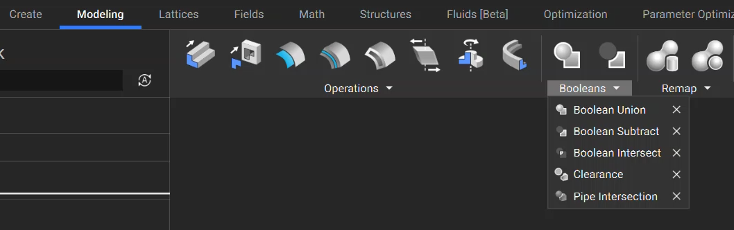
Boolean Blocks
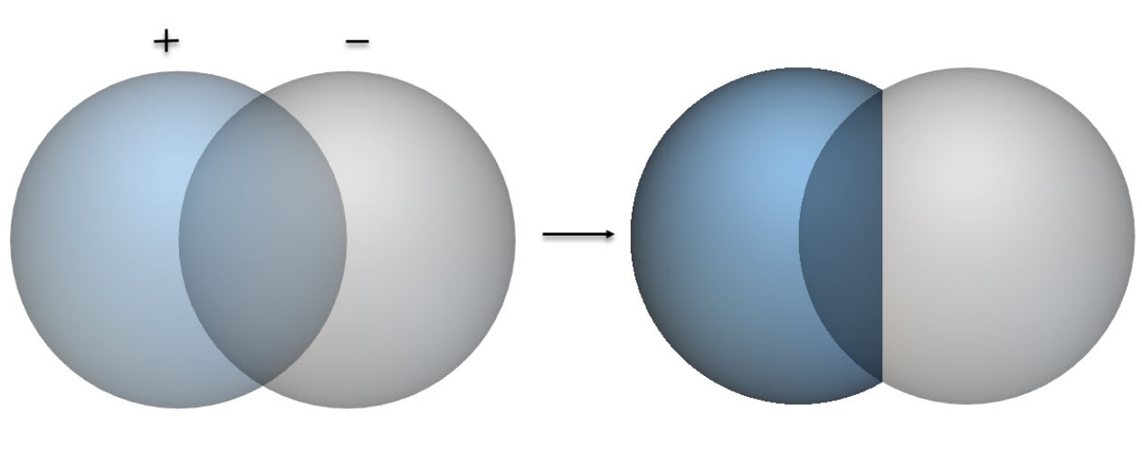
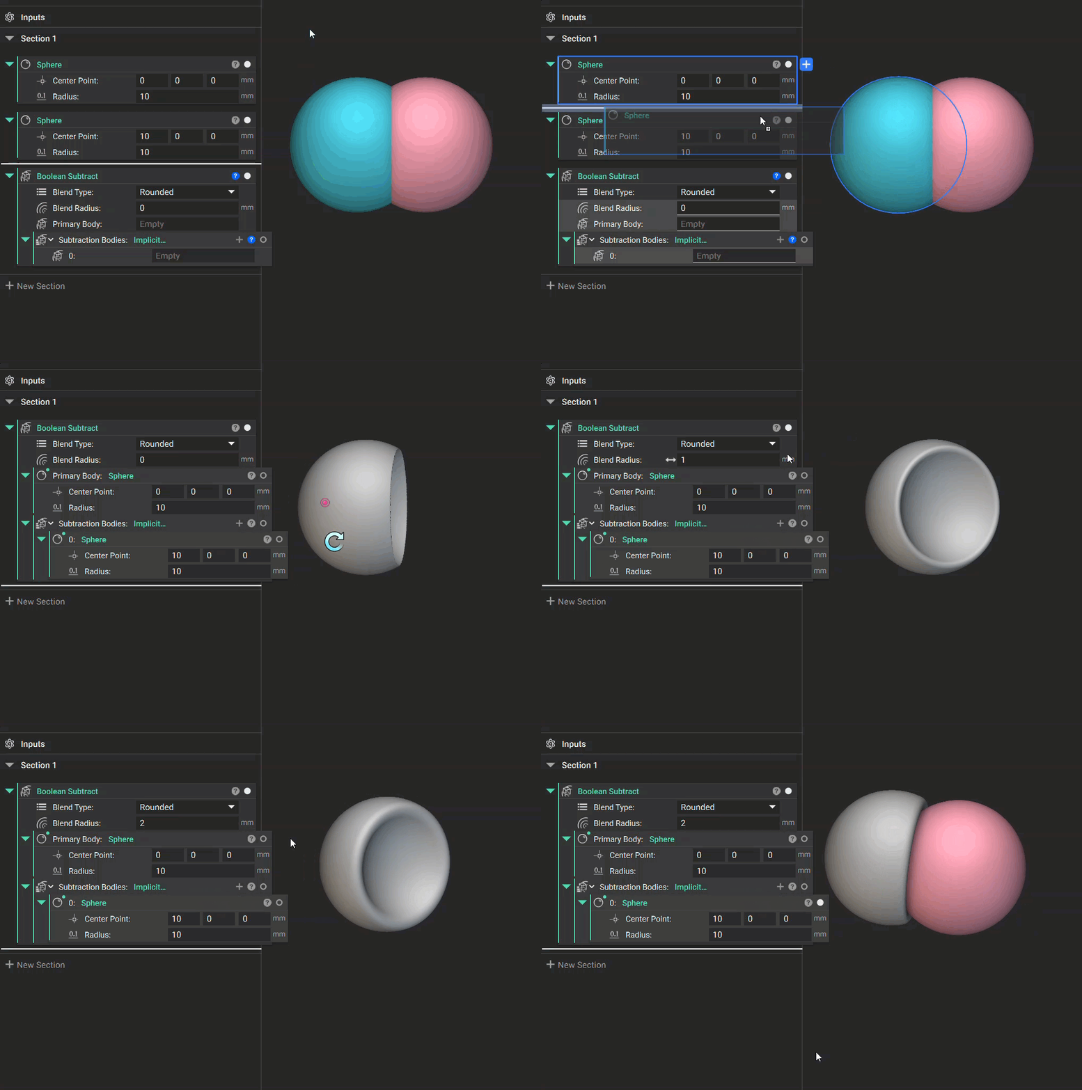
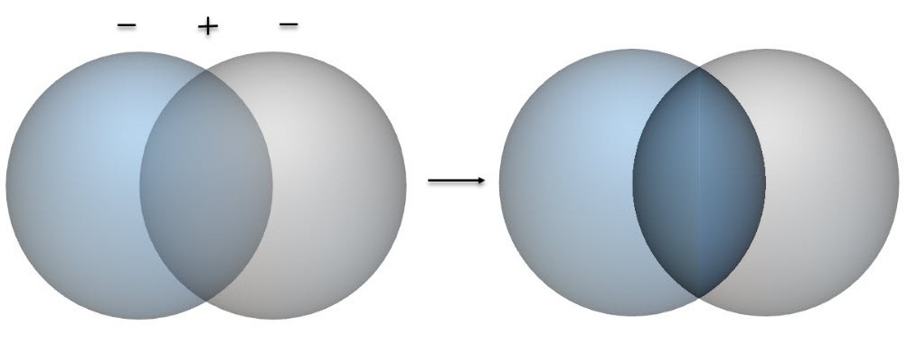
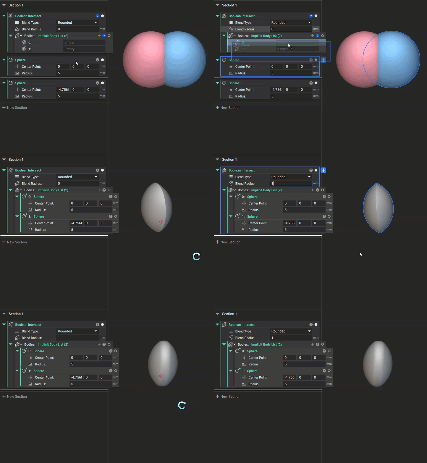
Boolean Union — Combines multiple Implicit Bodies into a single body, with an optional blend feature between the joining bodies.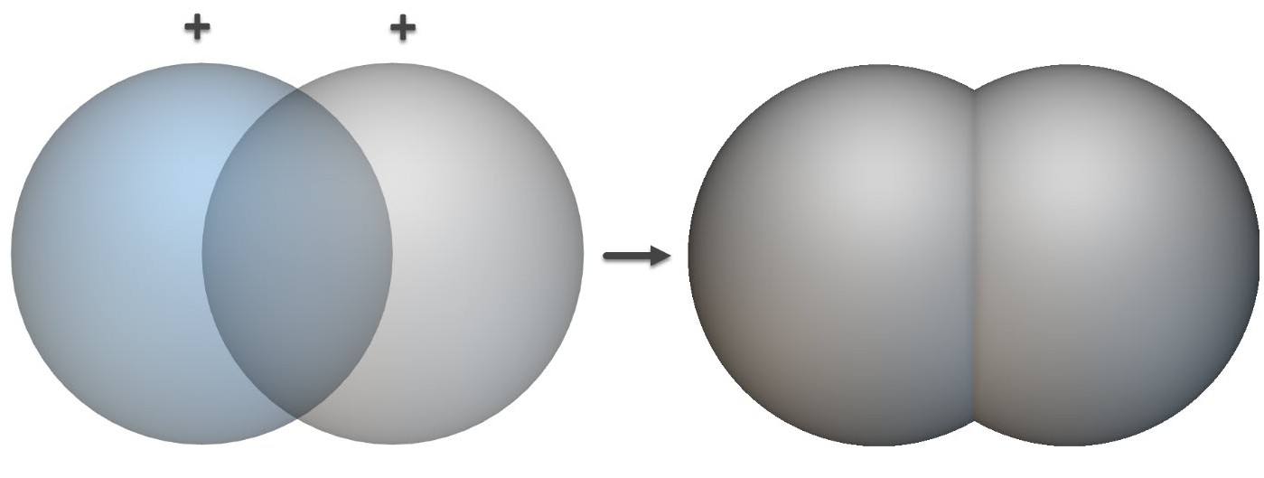
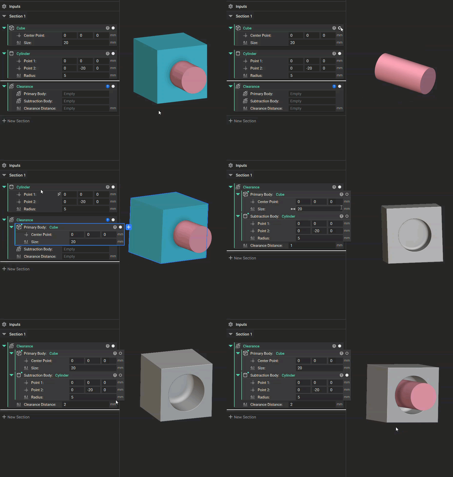
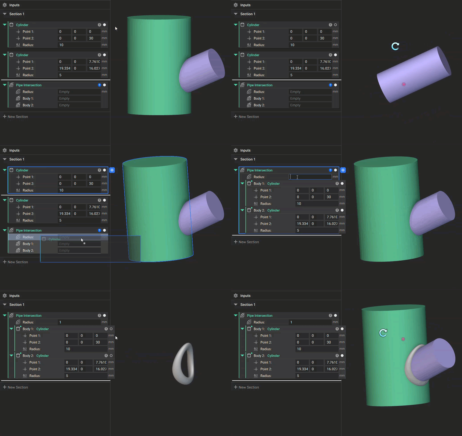
Blend Type
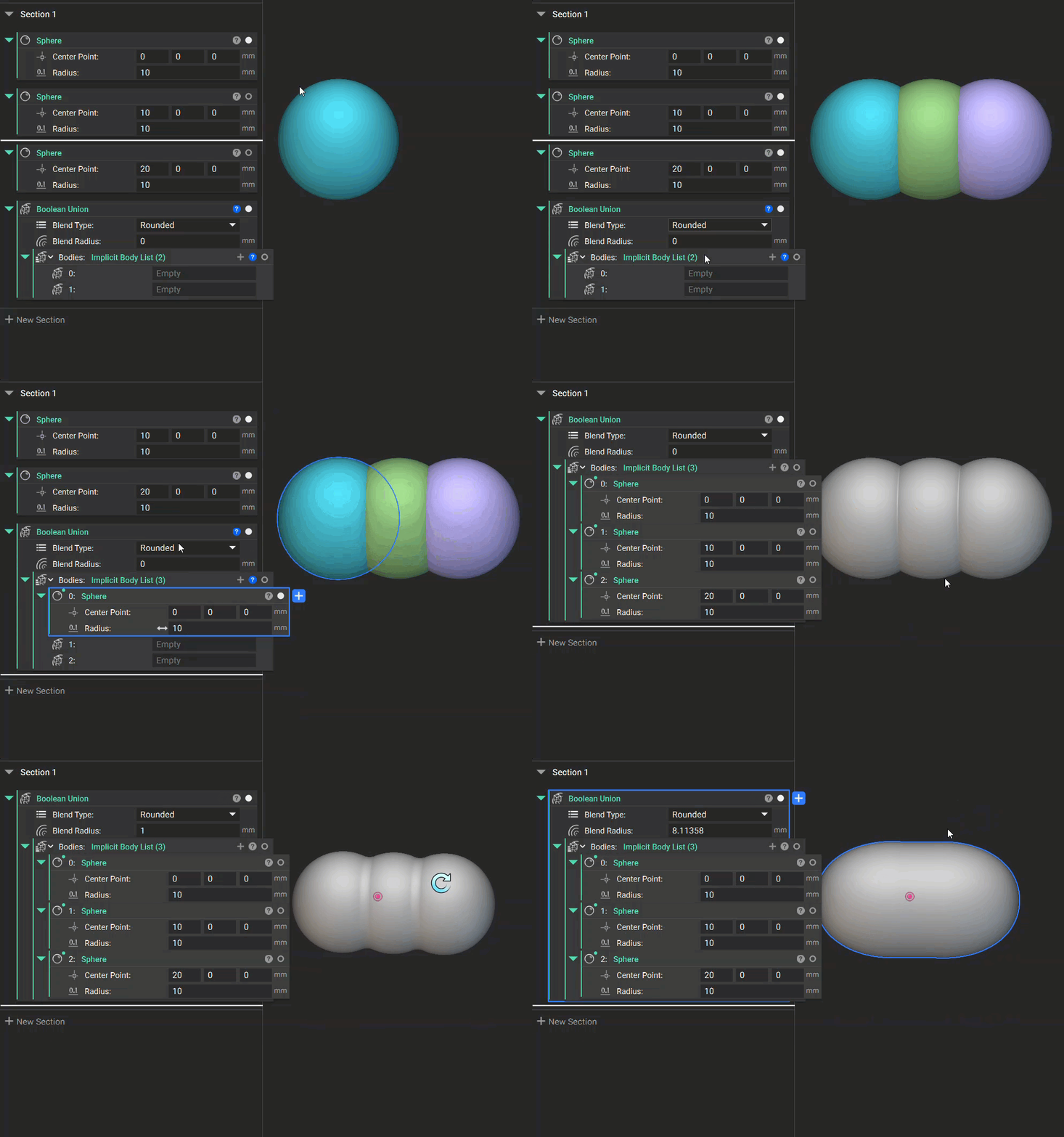
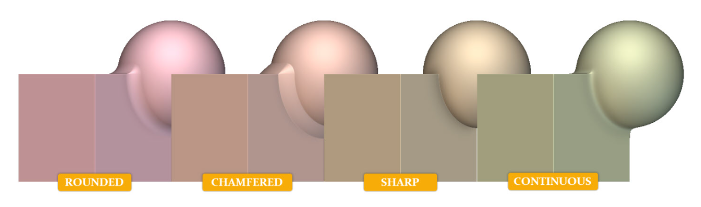
A blend can be applied where the input bodies intersect to control the transition between their volumes. The available Blend Types are:- Sharp preserves the original intersection without smoothing.
- Rounded creates a filleted transition.
- Continuous creates a smooth, curvature-continuous transition.
- Chamfered creates a beveled transition.
Cutting with a Plane
Splitting, cutting, and trimming are all accomplished the same way in nTop: by performing a Boolean Subtract or Boolean Intersect with a plane. This works because a plane defines more than a flat surface—it divides all of space into two infinite half-spaces. As established earlier in this lesson, the plane’s field is:- Zero on the plane itself
- Positive on the side toward which the normal points
- Negative on the opposite side
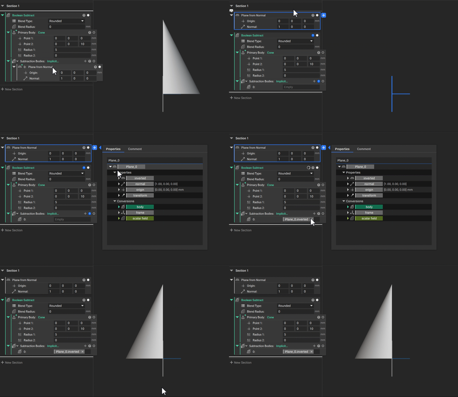
- Add a Plane or Plane from Normal block, both located in the Create tab under Vectors. A Plane is defined by an origin point and two in-plane axis directions; a Plane from Normal is defined by an origin point and a normal vector.
- Add a Boolean Subtract block from the Modeling tab.
- Assign the body to be cut to the Primary Body input.
- Assign the plane to input “0” of the Implicit Body List. You can use the plane directly here because the Plane type exposes a Body property that nTop reads as an implicit body.
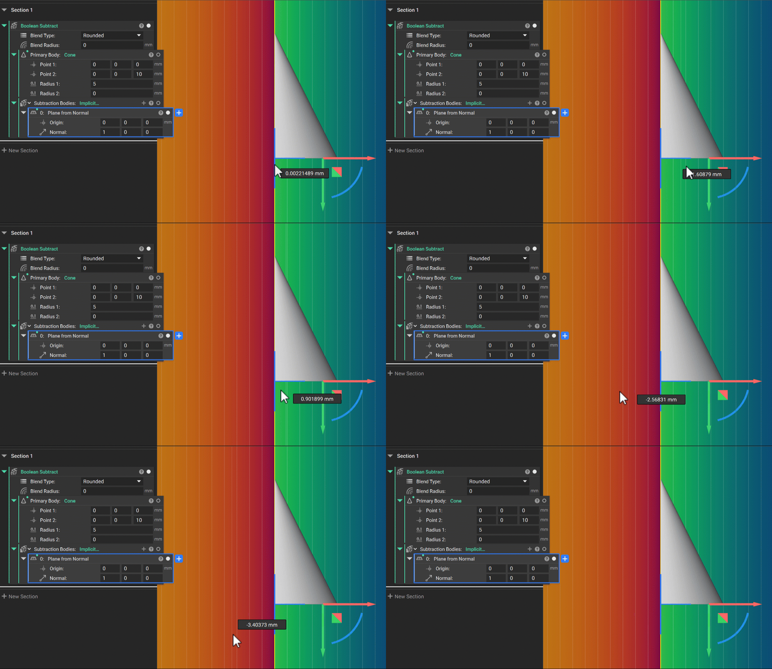
- Reverse the normal vector. In the Plane from Normal block, negate the normal—for example, change [0, 0, 1] to [0, 0, −1].
- Use the plane’s Inverted property within the Block Properties. This returns the same plane with its normal reversed.
What to Take Away
- A signed distance field assigns every point in space a value whose sign indicates whether the point is inside or outside a body and whose magnitude represents the distance to its surface.
- Fields extend infinitely through space. A bounding box defines the region that nTop evaluates and displays without changing the underlying field.
- The Viewport displays a sampled visualization of the field’s zero isosurface. Display resolution affects visual fidelity, not the underlying geometry.
- The Field Viewer allows you to inspect field values, isosurfaces, and potential defects. Evenly spaced, surface-parallel isolines indicate a healthy signed distance field.
- Boolean operations combine fields arithmetically, making unions, intersections, subtractions, and blends more robust than topology-based operations in traditional CAD.
- A plane’s field divides space into positive and negative half-spaces, allowing it to cut an implicit body through a Boolean Subtract or Intersect operation.