


What is a Field?
In Course 1, we learned that a field is a rule that assigns a value to every location in 3D space. When those values are numbers or scalars, the result is a scalar field. A scalar field can be described by a mathematical function, F(x,y,z), that returns a numerical value at each point P=(x,y,z). Fields are not limited to scalar values. A field can also assign a vector to each point in space, producing a vector field. Weather provides a familiar example of both. Temperature and humidity are scalar fields because each location is associated with a single numerical value. Wind velocity is a vector field because each location has both a wind speed and direction.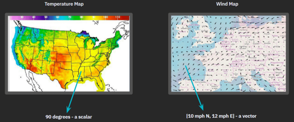
Fields in nTop
It can be helpful to think of fields as gradients for geometry. Just as a gradient controls how color varies across an image, a field in nTop controls how a design variable changes across space. The examples below illustrate this relationship using a signed distance field, field-driven geometry, and a color gradient. In the geometry example, the field controls the pattern and diameter of holes across a plate based on their spatial position. Similarly, the radial gradient controls how the grayscale value changes with distance from its center.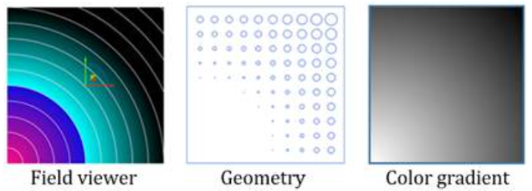
Why Use a Field Instead of a Constant?
A constant applies a single value uniformly. In nTop, many parameters can instead be driven by a field, allowing their values to vary continuously across a design. This enables two important capabilities: driving geometry from spatial data and controlling how design parameters vary throughout space.Drive Design with Spatial Data
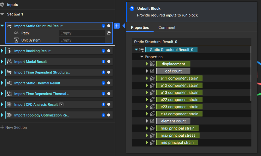
Fields can be derived from more than geometry. They can also come from simulation results, physical measurements, or imported datasets, allowing design parameters to respond directly to spatial data. For example, a Von Mises stress field from a structural simulation can drive rib thickness and density—creating thicker, denser ribs in regions of higher stress and thinner, less dense ribs in regions of lower stress. Rather than manually defining these parameters, the geometry adapts continuously to the underlying stress data.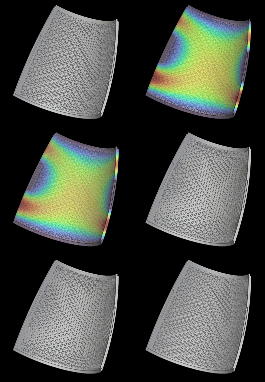
Control Spatial Variation
Fields are also useful when no external dataset is involved. A field can define how a parameter varies smoothly across a part based on position or other geometric relationships. The next section explores different methods for creating and controlling these variations. For example, a field can gradually increase shell thickness toward an edge, vary a Boolean blend radius across a transition, or control the progression from one profile to another. Instead of dividing the design into regions with individually defined constants, a single field can describe the variation continuously.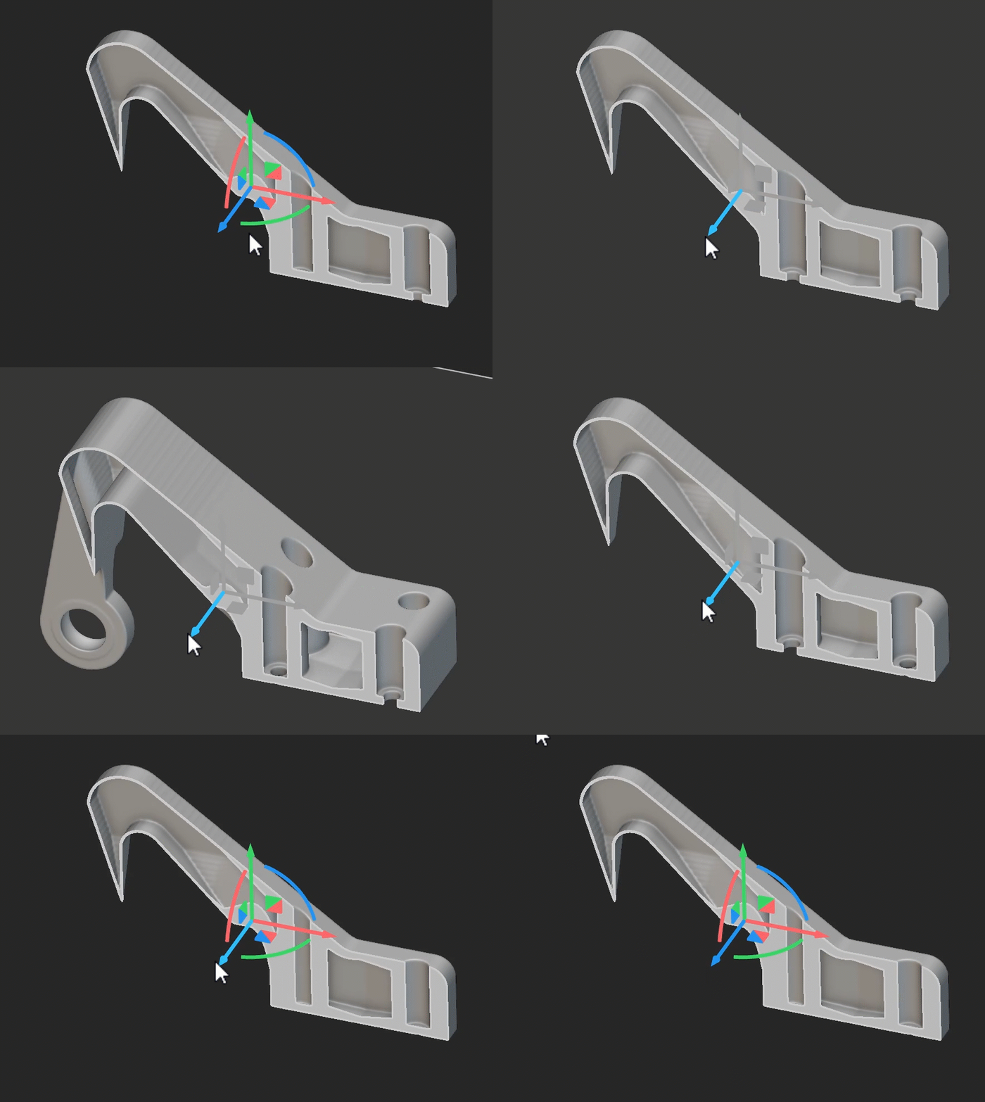
Creating and Controlling Fields
Now that you understand why fields are useful, the next step is learning how to create and control them. In this section, you will explore several approaches for defining fields in nTop and learn key tools for shaping their spatial variation. These techniques provide precise control over any compatible parameter identified by the Scalar Field symbol, enabling a wide range of field-driven design strategies.Extracting Distance Field of Implicit Bodies
Imported CAD or Mesh bodies do not have associated fields. However, converting them into implicit bodies generates distance fields. This means you can use any implicit body’s geometry to drive your designs. You can use the implicit body itself as the scalar field input or use the Scalar Field chip in its Properties panel if you want to manipulate this field further.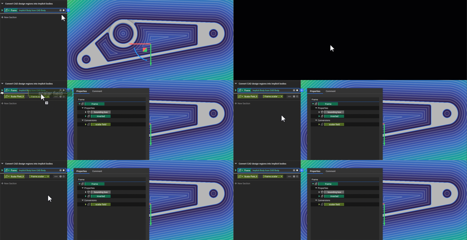
Using Equations
You can also manipulate and define fields with mathematical equations using the Scalar Field Variable block to create the x, y, or z variables. These represent the three axes and have fields that look like a plane set at the origin, with the normal direction in the positive direction of the axis.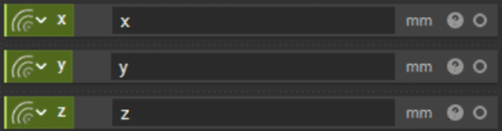
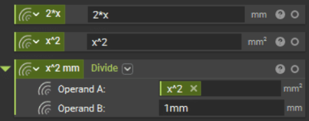
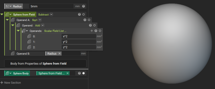
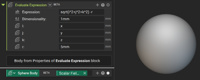
Converting Data or Images Into Fields
You can bring different types of data and even images into nTop, convert them into fields, and use them to drive your designs.Generating Fields from Data
You can import any dataset as point maps in CSV format using the Import Points, Import Table, Import Scalar Point Map, or Import Vector Point Map block, then interpolate it with the Field from Point Map block to get values at other points and form a field.Import Scalar Point Map & Import Vector Point Map
Import Scalar Point Map & Import Vector Point Map
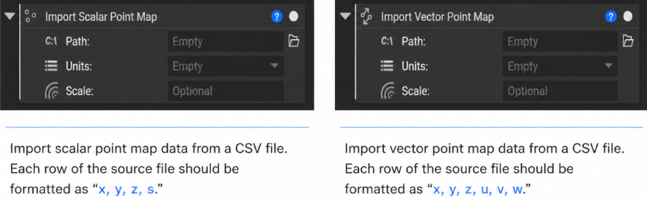
- Scalar Point Map: Each row contains four values: x, y, z, s. The first three define the point location; the fourth defines the scalar value at that point.
- Vector Point Map: Each row contains six values: x, y, z, u, v, w. The first three define the point location; the last three define the vector at that point.
- Units define the length units for point coordinates.
- Scale scales imported values and lets you assign units.
- Do not include units directly in the .csv file.
Field from Point Map
Field from Point Map
The Field from Point Map block interpolates Point Map data to create a field. It produces a Scalar Field from a Scalar Point Map or a Vector Field from a Vector Point Map.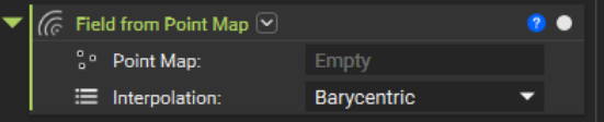 The Field from Point Map blockA common use of this block is to convert simulation results into a field, allowing simulation data to drive geometry modifications directly.
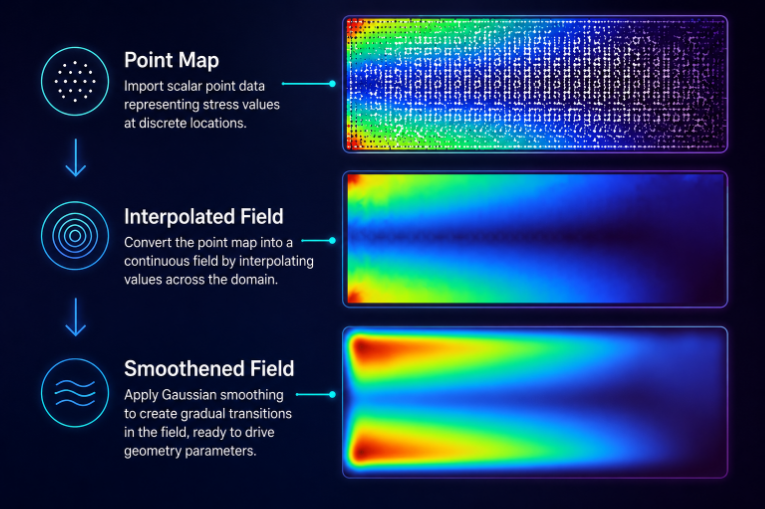
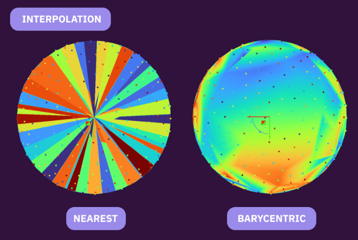 Comparison of Nearest and Barycentric interpolation applied to the same Point Map data, showing the discrete regions produced by Nearest interpolation and the smooth, continuous field produced by Barycentric interpolation.Because the resulting field will drive geometry, smoothing can create more gradual transitions between field values.
- Use the Field Viewer (F) to visualize the resulting field.
- Collinear or coplanar Point Map data cannot be interpolated; in these cases, the block extrapolates values.
- Choose an interpolation method based on the source data:
- Nearest: Assigns each location the value of its nearest Point Map point.
- Barycentric: Linearly interpolates values using surrounding points that form a tetrahedron. This method is recommended for Point Maps derived from tetrahedral meshes, such as Von Mises Stress Point Map or Temperature Point Map.
Smoothen Field
Smoothen Field
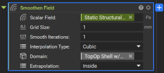
- Scalar Field — The field to smooth.
- Grid Size — The spacing between sample points used to discretize the field. Smaller values preserve finer detail but increase computation time.
- Smooth Iterations — The number of times the smoothing operation is applied. More iterations produce greater smoothing but increase computation time.
- Interpolation Type — The interpolation method used between sampled values: Linear or Cubic.
- Domain — An optional bounding box that defines the region to smooth. If you don’t specify a domain, the block uses the input field’s bounding box. Large domains may significantly increase computation time.
- Extrapolation — Controls smoothing relative to the specified Domain. Select Inside to constrain smoothing to the domain or Outside to extend smoothing beyond it.
- The Smoothen Field block requires a discretized field. The Grid Size controls the sampling resolution; smaller values capture finer detail but require more computation.
- Increasing Smooth Iterations produces a smoother field but also increases computation time.
- Balance Grid Size and Smooth Iterations to achieve the desired smoothness without unnecessary computational cost.
Note: The Smoothen Field block does not work on fields with infinite negative domains. You can remedy this by entering a Bounding Box in the optional Domain input or by first using Set Field Bounding Box on the field before inputting it into Smoothen Field*.*
Bitmapping Images
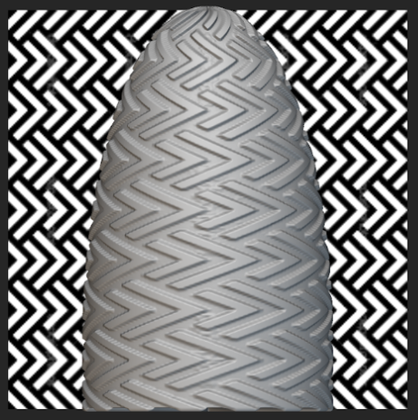
Bitmapping uses image data to drive design features, such as surface textures or logos. Import an image using the Import Bitmap block, then visualize and position it with Map Bitmap to Plane. The original image dimensions are available in the imported bitmap’s Properties panel. Use the Length and Width inputs to scale the image proportionally or independently to distort its proportions.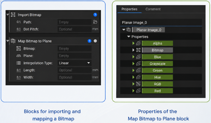
Tools for Working with Fields
When working with fields, three blocks are used most frequently. All are located in the Math tab under Utilities. Expand the sections below to learn about the fundamental Ramp, Transfer Function, and Mix blocks.Ramp Block
Ramp Block
The Ramp block allows you to change a value based on a field. It can be applied to several types of scalar fields and allows you to rescale those existing fields to create new ones.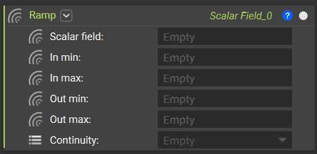 The Ramp block
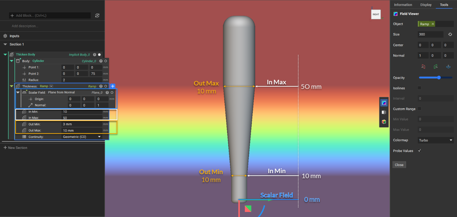 In this example, a plane was used for the Scalar Field input to create the gradual linear change seen between the start and end of the Ramp.
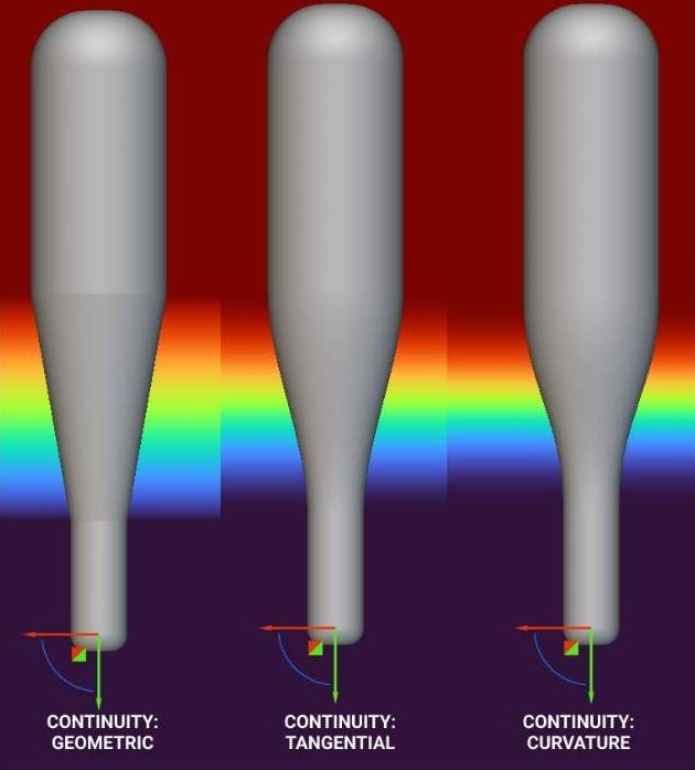 Visualization of the three different continuity options: Geometric (C0), Tangential (C1), and Curvature (C2)The change does not always have to be linear, depending on the field used. For example, if you use the field of x2 to drive the Ramp block, you would get a quadratic change. See this article on the Help Center for a walkthrough on creating a quadratic Ramp.
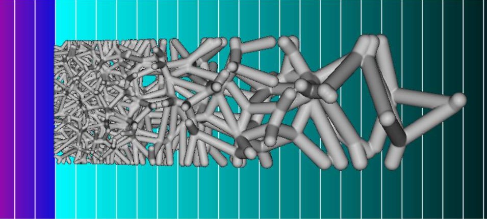 Manipulating density and beam thickness of a Voronoi lattice based on the field of a planeThis image shows the ramped lattice structure overlaid on the modifying field. The field modifies the seed point spacing and lattice thickness parameters.
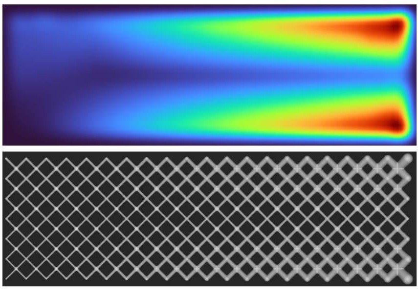 Manipulating lattice beam thickness based on simulated stress data that has been converted into a field and smoothenedThe lattice beams were assigned a larger thickness value at areas of higher stress and a smaller thickness value at areas of lower stress.
- Scalar Field: The field driving the Ramp. Define the In Min/In Max values based on this input.
- In Min/In Max: The values where the Ramp will begin (min) and end (max). These values are in relation to the Scalar field (with 0mm being the neutral edge of the field). Negative values go inside the Real Field, and positive values expand.
- Out Min/Out Max: The Ramp output values. Out Min is the output value at the In Min locations, and Out Max is the value reached at the In Max locations. They are the output field’s values as a function of the Scalar Field input.
- Continuity: Represents how the values will Ramp (by continuity order). See the image below to view the differences.
Note: Include units when defining the Out Min/Out Max values .
Note: Use the Field Viewer to visualize the new field created by the Ramp block by selecting the block and using the hotkey ‘F’. The new field will represent the output values assigned based on the spatial variation of the input field, which can then be used to control different design parameters.
Example Applications
Transfer Function Block
Transfer Function Block
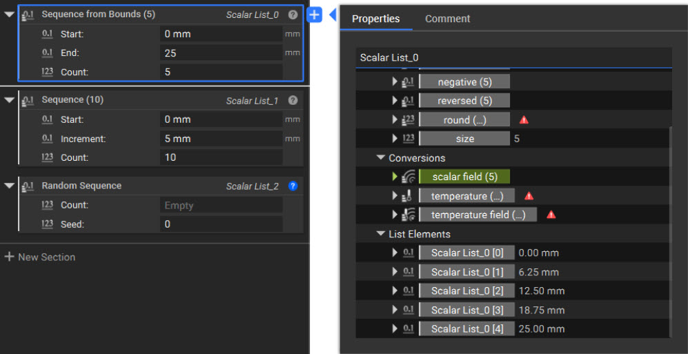
The Transfer Function block works very similarly to multiple mini ramps put together. This block gives you more control over the changes throughout the domain.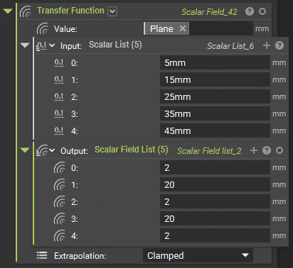 An example setup of the Transfer Function blockInstead of taking in minimum and maximum input and output values like the Ramp block, the Transfer Function requires lists of values as it uses piecewise interpolation to compute the output field value of a function approximated by a set of field data points.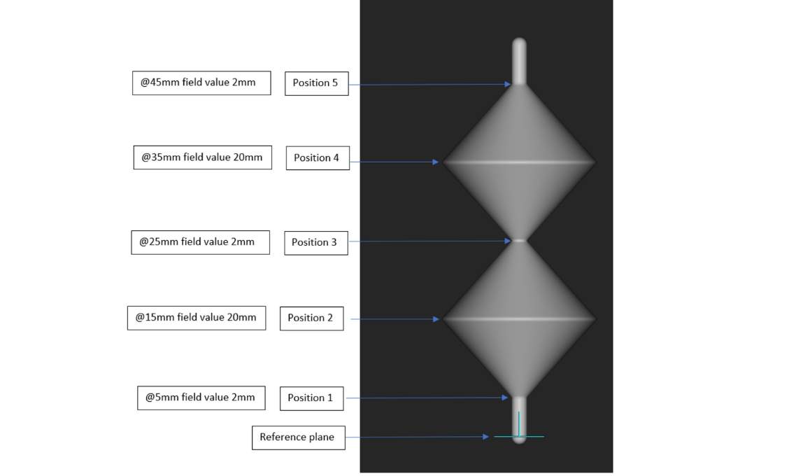
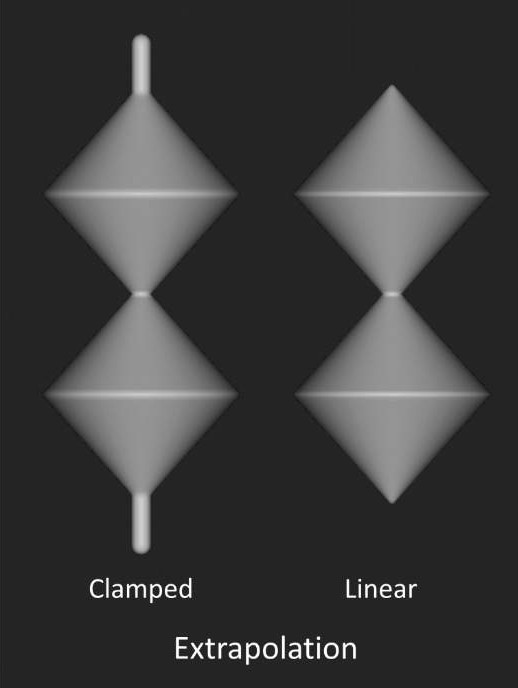 Example of the two extrapolation options
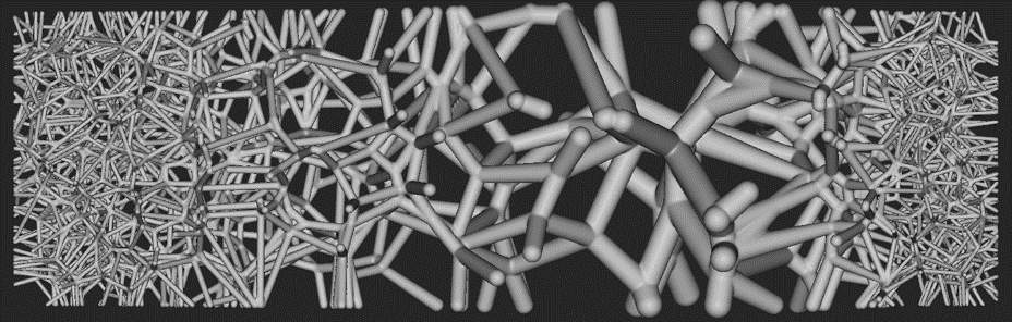 Advanced manipulation of beam thickness and density of a Voronoi lattice using a Transfer Function
- Value: The field driving the Transfer Function, a reference for the input domain.
- Input: Pre-populated as a Scalar List for a user-defined set of values.
- Output: A Scalar Field List of output values. The length of this list should match the length of the Input list.
Note: When defining the Input and Output values, make sure toinclude units**.
- Extrapolation: How the output values extend beyond the specified input domain. See the image below for a comparison of the two options.
- Clamped: Bounding output values remain constant beyond the specified domain
- Linear: Linear extrapolation of output values beyond the specified domain
Example Application
Mix Block
Mix Block
The Mix block is a tool for blending two implicit geometries by mixing the values of their scalar fields based on a given factor.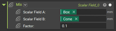 An example setup of the Mix block to mix a Box and ConeThe Factor value can range between 0 and 1, with 0 being entirely Input A and 1 being entirely Input B. The image below shows the effect of mixing a Box (Scalar Field A) and a Cone (Scalar Field B) using varying mix factors.
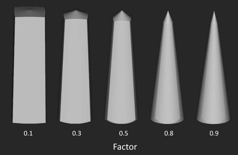 A comparison of the Mix block outcomes with varying Factor valuesThe Factor can also be ramped using the previously introduced Ramp block. See the example below with the same Box and Cone geometries.
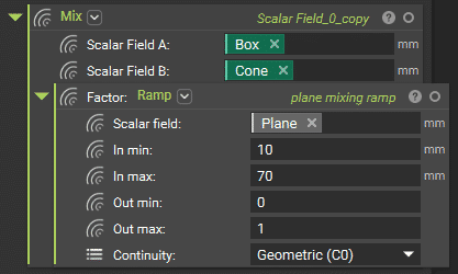 Applying a Ramp block to the Factor input of the Mix block
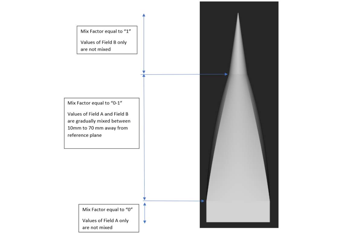 A diagram of the Mix block results with the ramped Factor input
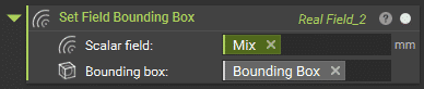 Applying a Set Field Bounding Box block to the Mix block
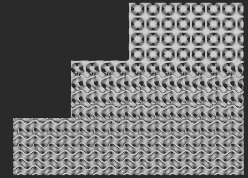 Gradually blending two types of TPMS latticesStarting with the Gyroid at the bottom, a Ramped Mix was applied to gradually blend the structure with the Neovius lattice.
Best Practice
Because the Mix block performs operations on two fields to represent a new geometry, it is always a good idea to perform a clean-up step afterward. This ensures that the resulting field does not have an infinite negative domain, which you cannot render into a geometry.Using the Set Field Bounding Box block, either manually set a bounding box using the Bounding Box block or go into the properties of the initial design body and grab its Bounding Box chip. The resulting field is within the specified bounding box.Example Application
What to Take Away
- Field-driven design replaces a uniform constant with a spatially varying field, enabling parameters such as thickness, displacement, blend radius, and pattern dimensions to change throughout a design.
- Fields may assign either scalar values or vectors to locations in space. Inputs that accept field-driven values are identified by the Scalar Field icon.
- Fields can be created from implicit-body distance fields, mathematical equations, simulation results, imported point maps, or bitmap images.
- Use the Field Viewer to verify a field’s values and spatial behavior before using it to drive geometry.
- Carefully manage units, scale, interpolation, and field domains when importing or constructing fields to ensure predictable results.