

Introduction
Engineering data rarely begins and ends in one application. nTop can import tabular data, meshes, and computer-aided design (CAD) geometry, then convert each source into a representation suited to downstream modeling or analysis. It can also export calculated results for use in other engineering tools. In this lesson, you will import coordinates from a comma-separated values (CSV) file and turn them into a closed airfoil shape. You will calculate its area and export the result. You will also import mesh and CAD versions of the same bracket, convert each for downstream modeling, and verify how units, source quality, and conversion settings affect the result.Understanding External Data in nTop
External data enters nTop as a specific data type. A CSV file can store ordered coordinates, a mesh represents surfaces with discrete faces, and CAD geometry represents boundaries with mathematically defined curves and surfaces. These source data types are not interchangeable, and they determine which blocks are available for immediate downstream operations. As discussed in previous lessons, many modeling operations in nTop use an implicit body. Converting imported geometry to this form makes it available to implicit modeling operations. The conversion is not a substitute for validation: units, point order, mesh quality, CAD detail, and conversion tolerance can all affect the result. The workflow in this lesson follows external data in both directions: source file to nTop representation to calculation to exported result.Create a Profile From CSV Coordinates
A closed profile is a filled planar region bounded by one or more closed curves. Coordinate-driven geometry follows a reusable pattern: import numeric values as points, connect the points into a curve, and convert the closed curve into a profile. An airfoil is a useful example because you can inspect each stage, but the same workflow applies to other closed planar shapes described by ordered coordinates. Please refer to the following files as you work through this section: Downloadable Files: Example File Download This file was last updated in nTop 6.03 CSV Example File: Airfoil CSV DownloadPrepare the CSV File
Use the provided airfoil CSV to follow the workflow, but structure the file as you would for any ordered point dataset: one point per row, three numeric columns in x, y, z order, and no header or metadata. For a closed profile, keep all z values equal, as the only way for the profile to remain closed is for the profile to remain planar.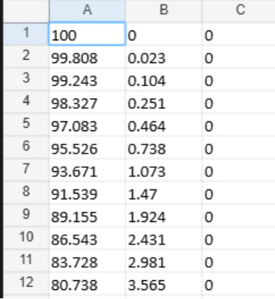
- Open the CSV file and confirm that every row contains three numeric coordinate values.
- Confirm the units used by the coordinate values. Assign these units when you import the file.
- Check for duplicated points and points separated by distances that are negligible for the intended geometry. Nearly coincident values can create unstable or self-intersecting curves.
- Inspect the first and last rows. They should describe the profile closure without creating a duplicated or nearly duplicated trailing-edge point.
Overview of the CSV to Profile Workflow
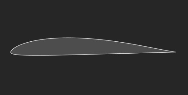
The workflow uses three standard blocks that you can add directly to any notebook. The custom block shown below packages them for convenience. In the reusable data path, the CSV values become points, the points define a spline, the periodic input closes the airfoil boundary, and the closed spline becomes a profile. For the custom block, the inputs are the airfoil root point, the airfoil CSV path, and the units. The main body contains a Spline Through Points block that processes the CSV points and a Profile from Curves block that converts the spline into a profile. The custom block outputs the airfoil profile generated from the CSV.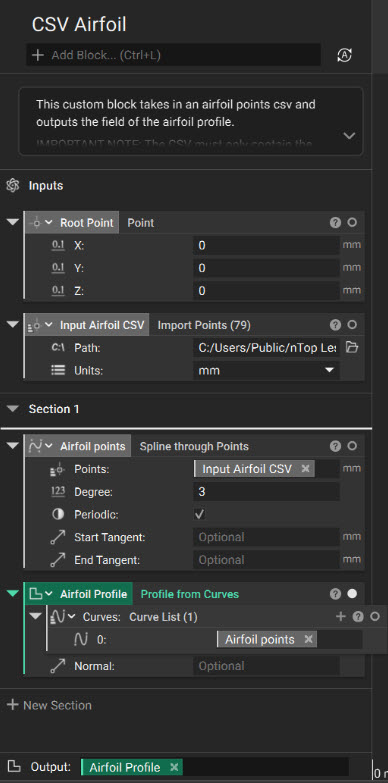
- Import Points reads coordinate rows from the Path input, interprets them using the Units input, and returns points.
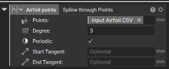
- Spline Through Points connects the Points input in row order. A spline is a smooth curve fitted through those points. Set Degree to 3 as a common starting point and enable Periodic when the boundary must close.
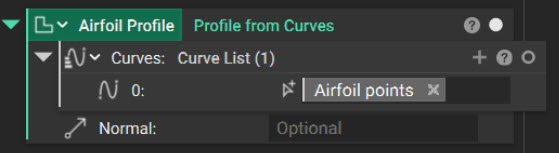
- Profile from Curves converts coplanar Curves into a planar profile. Correct an open, self-intersecting, or non-coplanar curve before this step.
Assemble the Workflow
- Add an Import Points block, select the CSV file with the Path input, and set Units to match the coordinate values.
- Add a Spline Through Points block, connect the imported points to the Points input, set Degree to 3, and enable Periodic for the closed boundary.
- Add a Profile from Curves block, connect the spline to the Curves input, calculate the workflow, and display the resulting profile.
Alternative Method: Import the CSV as a Table
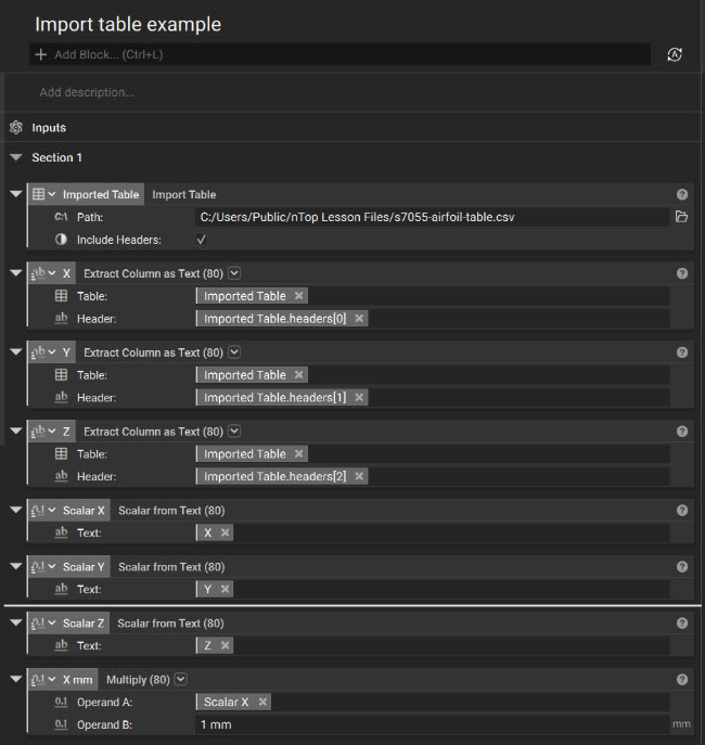
Import Points is the shortest path for a coordinate-only CSV without a header. The Import Table block is useful when the file has named columns or additional tabular values that you want to access independently. Please refer to the following files as you work through this section: Downloadable Files: Example File Download This file was last updated in nTop 6.03 CSV Example File: Airfoil Table Download For this alternate route, use a copy of the airfoil CSV with x, y, and z headers in the first row.- Add an Import Table block, select the headered CSV with the Path input, and enable Include Headers.
- Add three Extract Column as Text blocks and assign the x, y, and z column headers to them.
- Connect each extracted text list with Scalar from Text. Multiply each resulting scalar list by 1 mm, or by the length unit used in the source file, so the coordinates carry units.
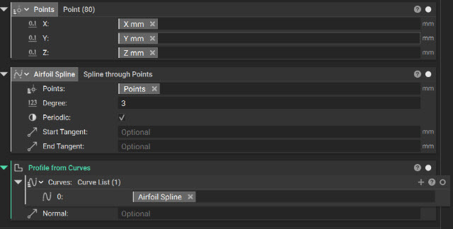
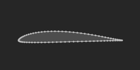
- Add a Point block and connect the unit-bearing scalar lists to its X, Y, and Z inputs. nTop list processing creates one point for each table row.
- Connect the point list using Spline Through Points, set Degree to 3, enable Periodic, and generate the profile from the resulting curve using Profile from Curves.
Verify the Resulting Profile
Before using imported data downstream, verify that nTop interpreted it as intended. Check that:- The profile occupies the intended region inside the boundary.
- The curve is smooth wherever the source data should be smooth.
- The profile closes cleanly at both the leading and trailing edges.
- No loop, spike, or unintended region appears outside the boundary.
Calculate and Export a Scalar Result
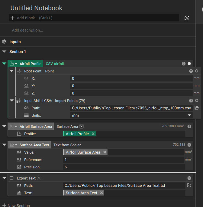
The Surface Area block accepts a profile, mesh, or implicit body and returns an area value. When you use the airfoil profile directly, the result is the enclosed area of the two-dimensional profile, not the exterior surface area of a three-dimensional wing. The result is a scalar: a single magnitude with an associated unit.Calculate the Surface Area
- Add a Surface Area block to the notebook.
- Set the Profile input of the Surface Area block to Airfoil Profile.
- Review the calculated value and its units.
Export the Scalar Value
nTop retains units as part of a scalar. A plain-text file does not retain nTop’s data type, so the value must first be formatted as text with an explicit reference and precision.- Add a Text from Scalar block and connect the area to its Value input.
- Set Reference to the desired area unit, such as 1 mm². The exported number will be expressed relative to this value.
- Set Precision to the number of significant digits needed by the downstream workflow.
- Add an Export Text block, connect the formatted value to its Text input, and choose the output Path.
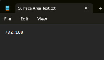
- Open the exported file and confirm that the number corresponds to the value displayed in nTop.
Import Mesh and CAD Geometry
Mesh and CAD files can describe the same physical part, but they represent its boundary differently. A mesh approximates the boundary with discrete faces. CAD geometry uses mathematically defined curves and surfaces. Converting either source to an implicit body gives subsequent implicit modeling blocks a common data type. The steps below use explicit import and conversion blocks so that each data-type change is visible. You can also drag supported files into nTop and access available conversion operations by right-clicking selected geometry. Please refer to the following files as you work through this section: Example Mesh: Mesh File Download Example CAD: CAD File DownloadImport and Convert a Mesh
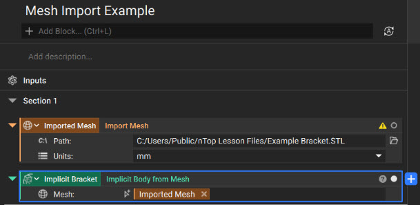
- Add an Import Mesh block, select the provided file with the Path input, and set Units to the units used when the mesh was exported. Alternatively, drag the mesh file into nTop, then confirm that the imported mesh uses the correct units.
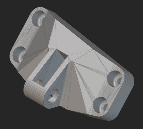
- Inspect the imported mesh for obvious holes or disconnected regions. In the Properties panel, confirm that it is closed, manifold, oriented, and not self-intersecting. Closed means no open boundary edges; manifold means each edge has an unambiguous surface connection; oriented means the face directions are consistent; and non-self-intersecting means no faces cross one another.
- Add an Implicit Body from Mesh block and connect the imported mesh to its Mesh input.
- Toggle the visibility of the mesh and implicit body, or use a section view, to compare their boundaries.
Import and Convert CAD Geometry
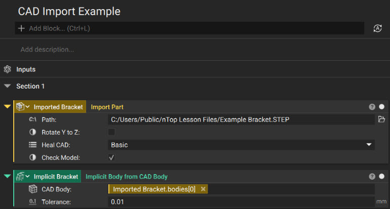
- Add an Import Part block and select the provided CAD file with the Path input.
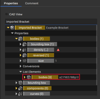
- Extract a single CAD body from the imported part. You can drag the individual body property into the notebook or use Get CAD Bodies when a block-based selection is more appropriate. Do not pass a CAD body list to an input that expects one body. Refer to the image below on where to find the body in the properties menu.
- Add an Implicit Body from CAD Body block and connect the selected body to the CAD Body input.
- Set the Tolerance to the maximum permitted deviation between the CAD source and the implicit result. Use a smaller value when the part contains important small features or thin regions.
- Compare the CAD and implicit boundaries to confirm that small features and thin regions were captured.
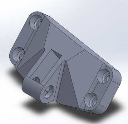
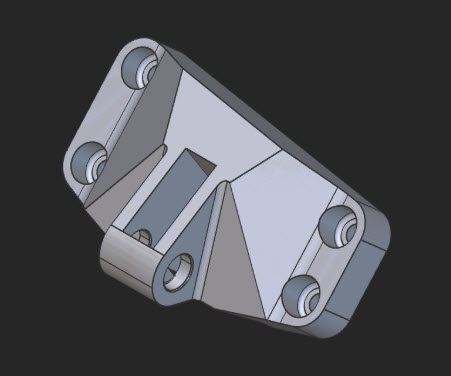
Compare the Data Paths
The three workflows produce nTop data types that can be used in downstream operations, but each has a different source of uncertainty:- CSV coordinates depend on formatting, units, point order, and clean profile closure.
- Mesh geometry depends on tessellation resolution and mesh topology.
- CAD-to-implicit conversion depends on the selected body and conversion tolerance.
What to Take Away
- External files enter nTop as specific data types, and those types determine which downstream operations are available.
- A coordinate CSV becomes geometry only after nTop interprets its values as ordered points, a curve, and a profile.
- Mesh and CAD geometry can both be converted to implicit bodies, but source quality and conversion settings affect the fidelity of the result.
- The Surface Area block returns a scalar value that can be formatted with controlled units and precision before export.
- Every imported or converted result should be checked before it is used downstream.